ftool¶

Interactive curve-fitting tool for 1D and 2D data. By default uses erlab.analysis.fit.models.MultiPeakModel, but you can pass any 1D lmfit model.

There are three ways to start ftool.

erlab.interactive.ftool()
```
import erlab.interactive as eri

eri.ftool(data)
```
To supply a custom model:
```
eri.ftool(data, model=my_model)
```
For a weighted fit, supply the absolute standard uncertainty of each data point:
```
eri.ftool(values, uncertainty=standard_uncertainty)
```
ftool displays these values as one-standard-deviation error bars and passes their reciprocal to lmfit as weights. The uncertainty may omit dimensions that xarray can broadcast from the data. Its coordinates must align with the data coordinates. Its values must be finite and positive where the data is finite.
From the ImageTool context menu

Right-click an image plot or line plot and choose ftool.
From IPython using the %ftool magic described in Notebook shortcuts.
```
%ftool data
%ftool --model my_model data
```

When ftool is opened from an ImageTool in the manager, it remembers the slice or line cut that opened it. If that ImageTool changes, the manager can update the tool from the latest compatible data. Enable Refit after update when the same fit should rerun after updates. For 2D fits, parameter maps opened in ImageTool appear as child rows under ftool.

Overview¶

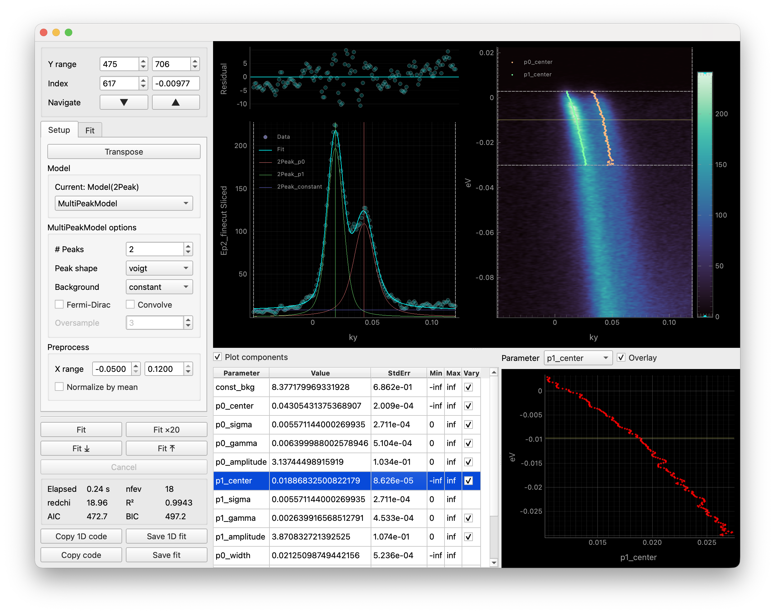
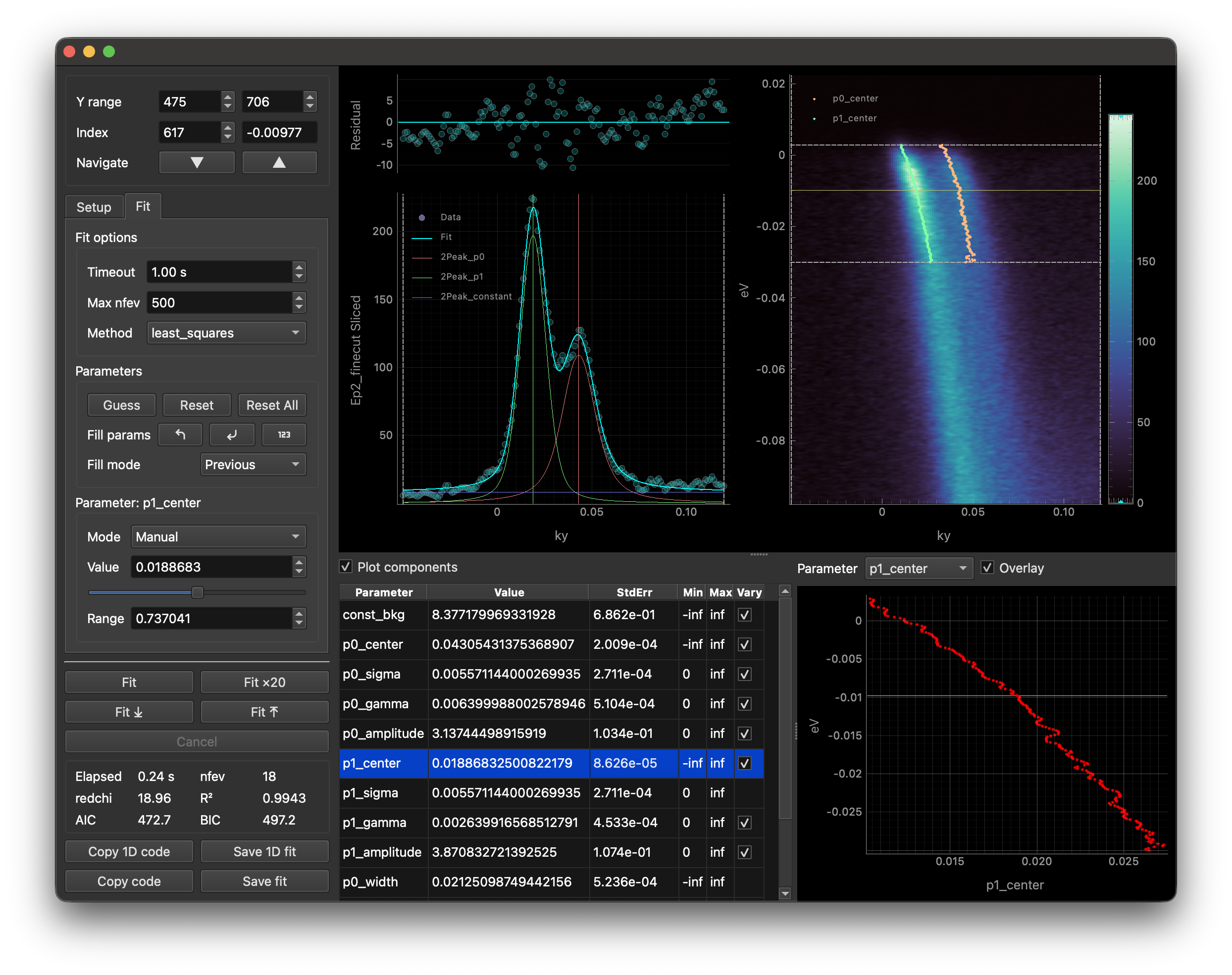
When you first open ftool, you will see a stack of controls on the left and a plot on the right, as shown below. The controls have two tabs: Setup and Fit.

Setup

Fit

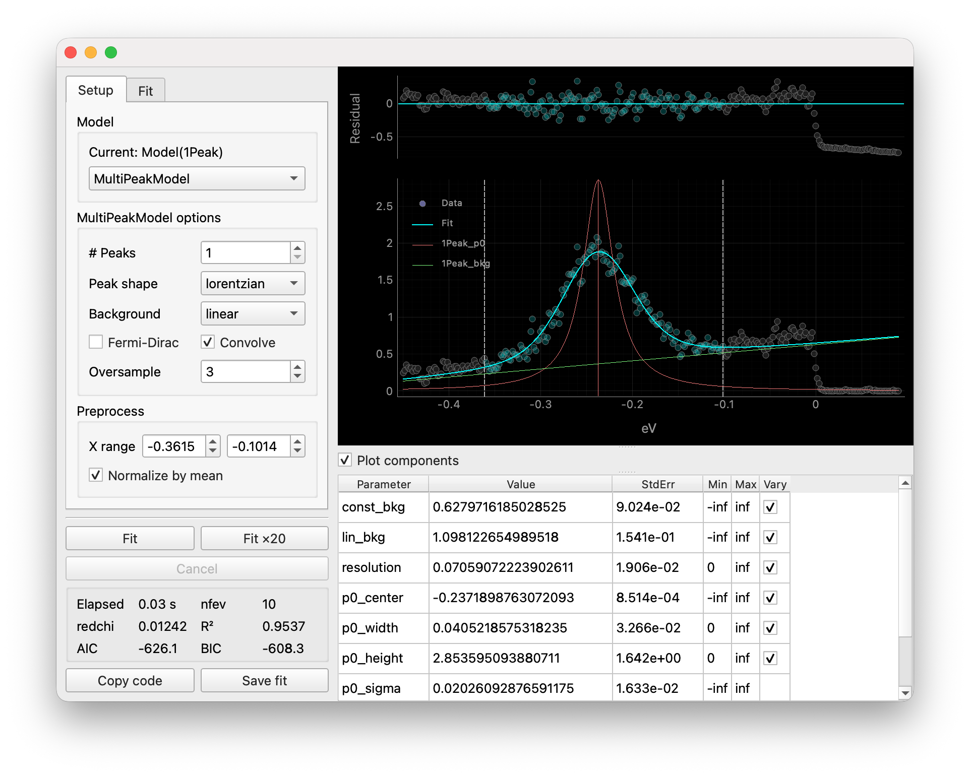
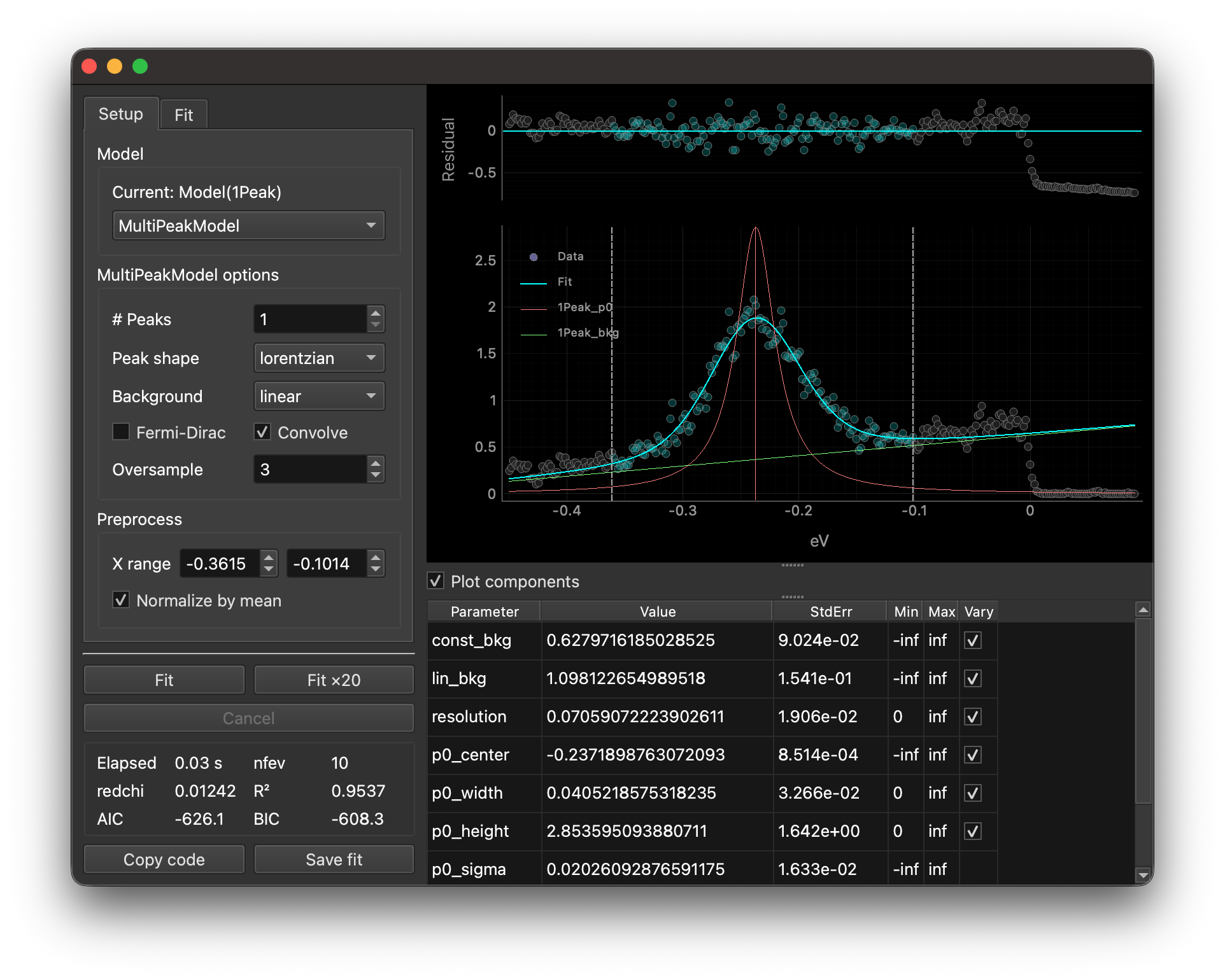
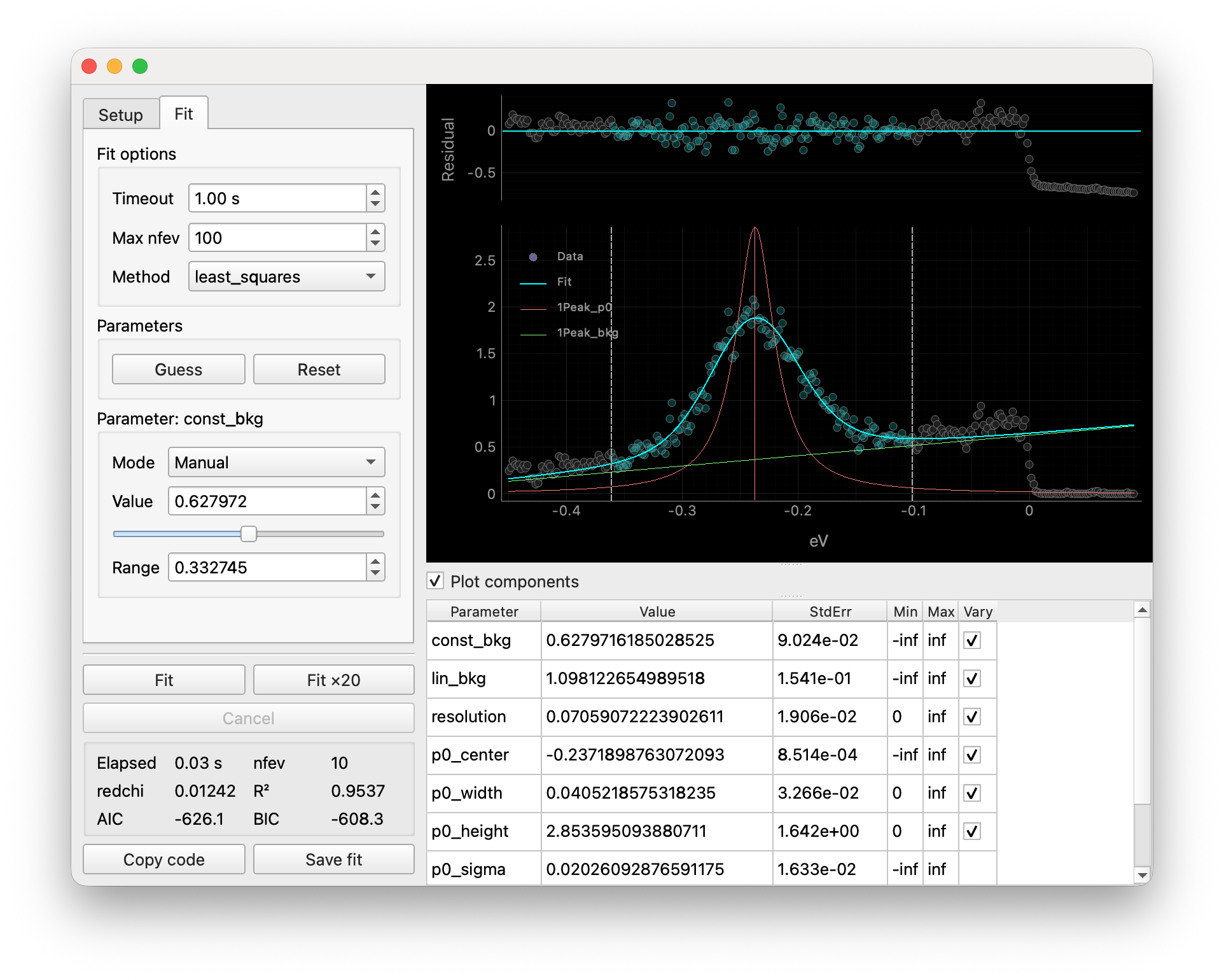
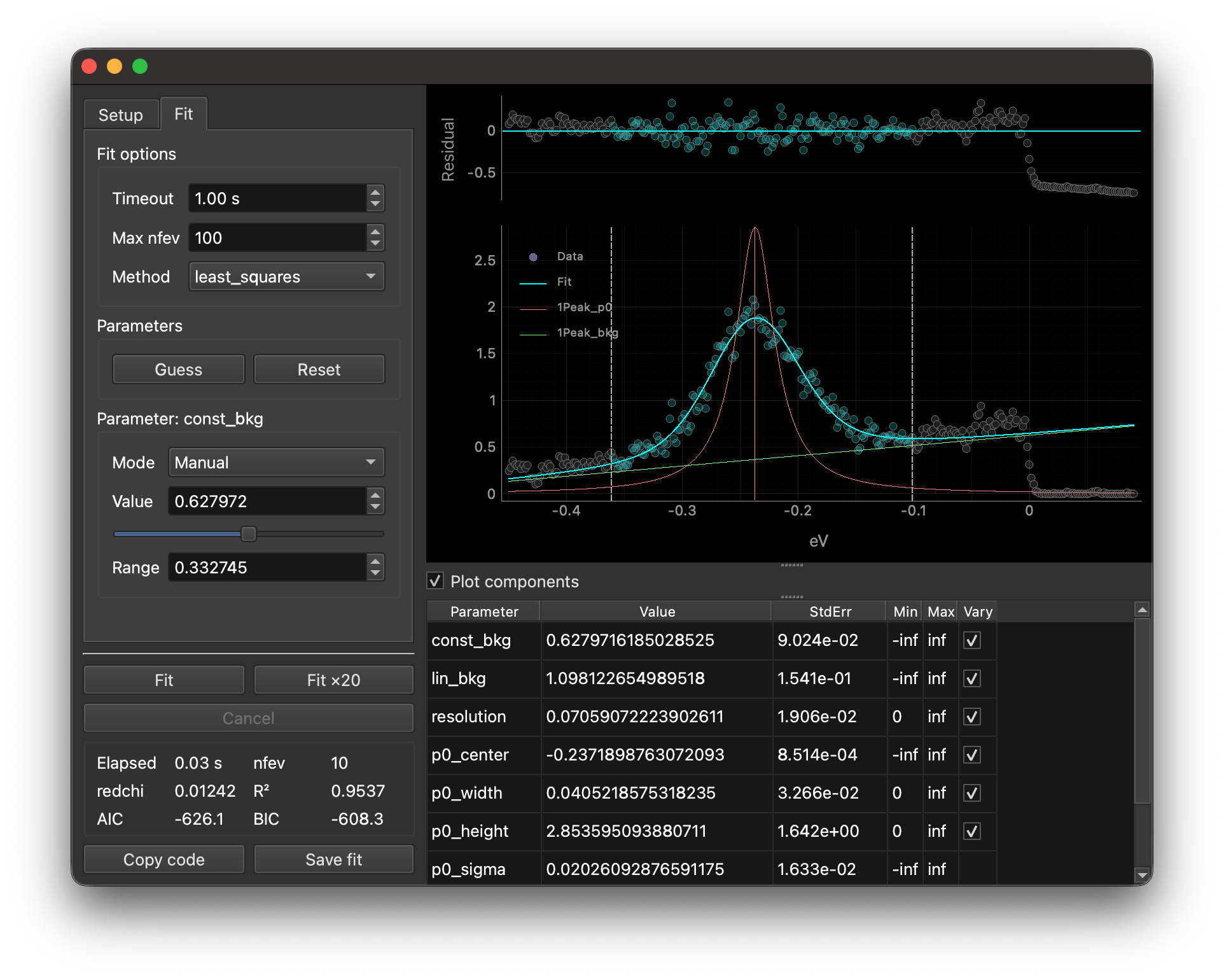
The main plot shows the data with the fit overlay, plus dashed vertical lines that define the current fit window.
- Check Plot components to show individual model components (if any). This also adds a legend for each curve. You can show/hide a component by clicking its legend entry.
The left panel contains controls for setting up and performing the fit. The Setup tab is for choosing the model and preprocessing options, while the Fit tab contains parameter settings and options related to the fitting process.

Models and options¶

First, use the Model drop-down to choose a predefined model, a user-provided model, or a model loaded from disk.

Built-in options are:
From file loads a lmfit model saved with lmfit.model.save_model().

Some models have additional options that appear below the model selector that are used to initialize the model:

MultiPeakModel:
- # Peaks and Peak shape define how many components are fit and whether they are Lorentzian or Gaussian.
- Background and Degree add a constant, linear, or polynomial background.
- Fermi-Dirac multiplies the peaks by a Fermi-Dirac distribution.
- Convolve applies instrumental broadening; Oversample controls the internal sampling density used for the convolution.
ExpressionModel:
- Edit the independent variable name in the f(...) header. Then type your formula, such as a * x + b, in the expression box.
- Click Apply to rebuild the model from the current expression.
- Use Edit init script… to define helper functions or constants used in the expression.
- For more information, see the documentation for lmfit.models.ExpressionModel.

For complete fitting procedures, see Fitting one curve.

Fit ×20 performs 20 consecutive fits on the same curve. Each fit supplies its fitted parameters as the starting values for the next fit. This can help a nonlinear or highly correlated model converge after one fit stops near a solution.

Two-dimensional input¶

For two-dimensional input, ftool shows an image, one selected curve, and a parameter-versus-coordinate plot. Transpose controls which dimension is the fitted coordinate. Index and the yellow cursor select the curve displayed in the fit panel.

When working in ImageTool Manager, open the parameter values in ftool to fit them using their standard errors. The weighted fit omits points without a finite, positive standard error. If no valid points remain, ftool does not open.

Setup

Fit

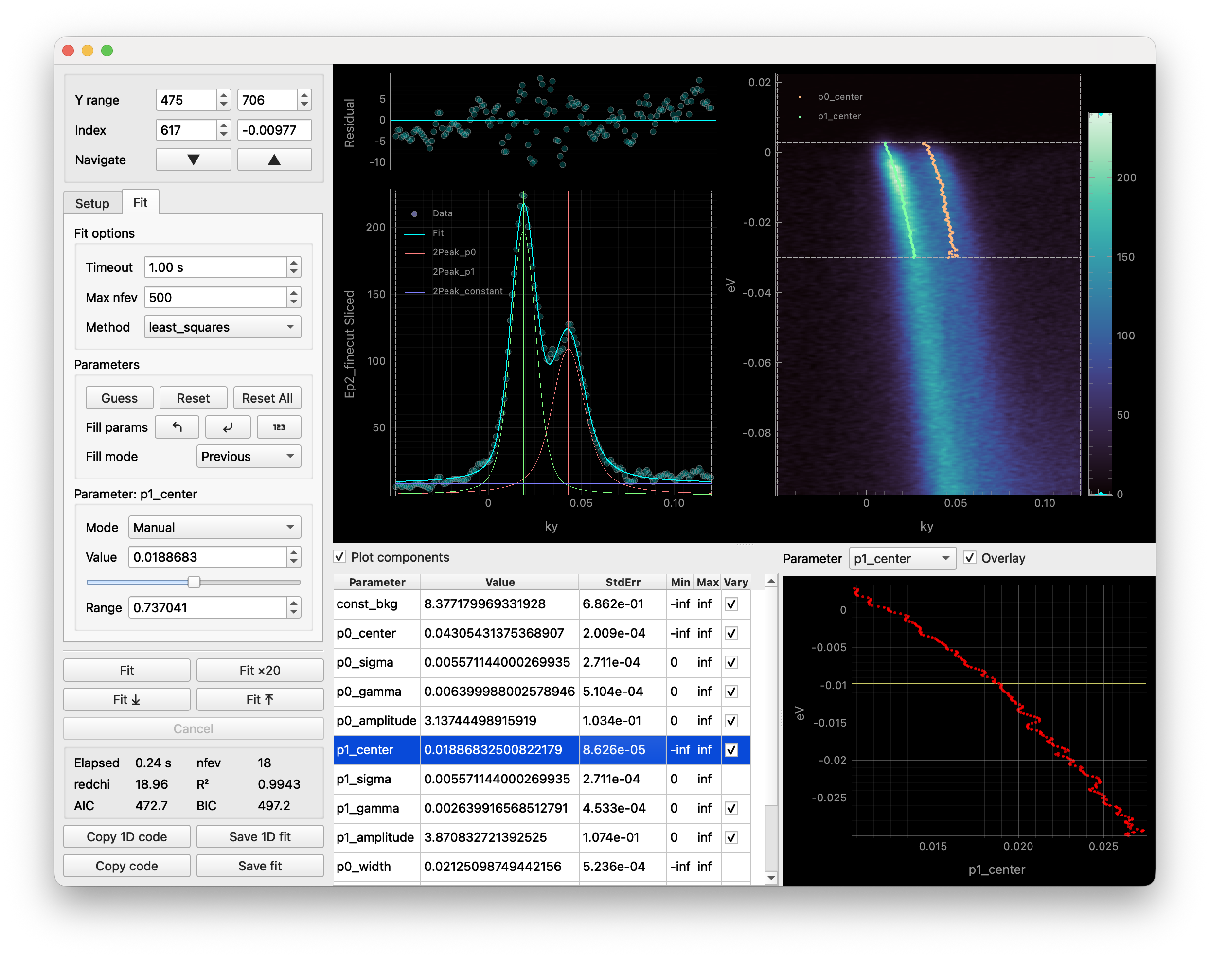
Fill mode controls parameter initialization during a fit sequence. Previous uses the last good fit, Extrapolate projects from the previous two fits, and None keeps the existing initial values.

For the work procedure, see Fitting a stack of curves.