Filtering

Image processing-related functions are commonly used in the analysis of ARPES data. The erlab.analysis.image submodule provides a collection of functions that are useful for processing and analyzing images.

The module includes xarray wrappers for several functions in scipy.ndimage and scipy.signal, along with several processing methods that are commonly used to visualize ARPES data.s

Image smoothing filters

import erlab.analysis as era

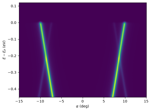
First, let us generate some example data: a simple tight binding simulation of graphene.

from erlab.io.exampledata import generate_data_angles

cut = generate_data_angles(
    shape=(500, 1, 500),
    angrange={"alpha": (-15, 15), "beta": (-5, 5)},
    seed=1,
    bandshift=-0.2,
).T
cut.qplot()

<matplotlib.image.AxesImage at 0x703cd951de80>

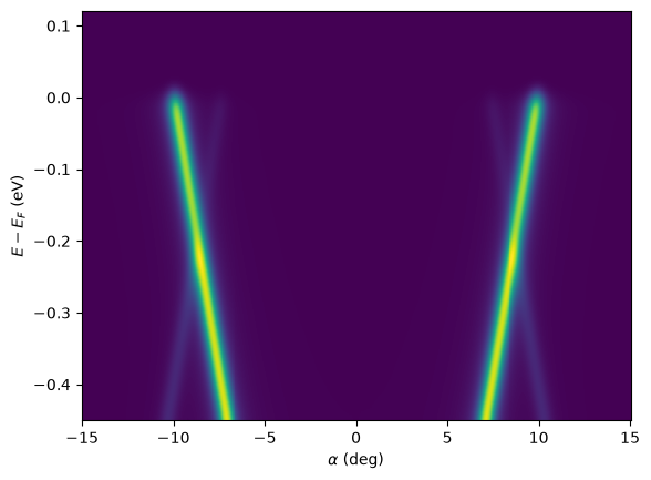
Here, we apply a Gaussian filter in coordinate units using erlab.analysis.image.gaussian_filter() to simulate an instrumental broadening of 10 meV and 0.2 degrees:

cut_smooth = era.image.gaussian_filter(cut, sigma=dict(eV=0.01, alpha=0.2))
cut_smooth.qplot()

<matplotlib.image.AxesImage at 0x703ccab80910>

For all arguments and available filters, see the API reference at erlab.analysis.image.

Visualizing dispersive features

Important

An interactive tool for smoothing and differentiation is available; see dtool for details.

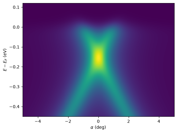
There are several methods that are used to visualize dispersive features in ARPES data. To demonstrate, we first generate a synthetic ARPES cut with broad features:

import erlab.analysis as era

from erlab.io.exampledata import generate_data_angles

cut = generate_data_angles(
    shape=(500, 1, 500),
    angrange={"alpha": (-5, 5), "beta": (-10, 10)},
    temp=200.0,
    seed=1,
    bandshift=-0.15,
    Simag=0.1,
    count=1e11,
).T
cut.qplot()

<matplotlib.image.AxesImage at 0x703cda1dfd90>

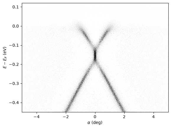
The 2D curvature can be calculated with erlab.analysis.image.curvature():

result = era.image.curvature(cut, a0=0.1, factor=1.0)

result.qplot(vmax=0, vmin=-200, cmap="Greys_r")

<matplotlib.image.AxesImage at 0x703ccaa65950>

For different methods and arguments, see the API reference at erlab.analysis.image.