Other interactive tools¶

In addition to ImageTool and the ImageTool manager, other interactive tools for specific tasks are available in the erlab.interactive module.

Most of these tools can be opened as auxiliary windows from within ImageTool, and are also integrated into the ImageTool manager, allowing you to manage them alongside your ImageTool windows.

More interactive tools will be added in the near future. Current plans include:

Fourier-based automatic mesh removal
Experiment planner

Here are some of the miscellaneous interactive tools provided:

ktool¶

Interactive conversion from angles to momentum space.

There are four ways to start ktool.

xarray.DataArray.kspace.interactive()
```
data.kspace.interactive()
```
erlab.interactive.ktool()

This option is recommended because the name of the input data will be automatically detected and applied to the generated code that is copied to the clipboard.
```
import erlab.interactive as eri

eri.ktool(data)
```
From within ImageTool

Click View → Open in ktool.

The button will be disabled if the data is not compatible with ktool.
From IPython using the %ktool magic described in Notebook shortcuts.

The GUI is divided into two tabs.

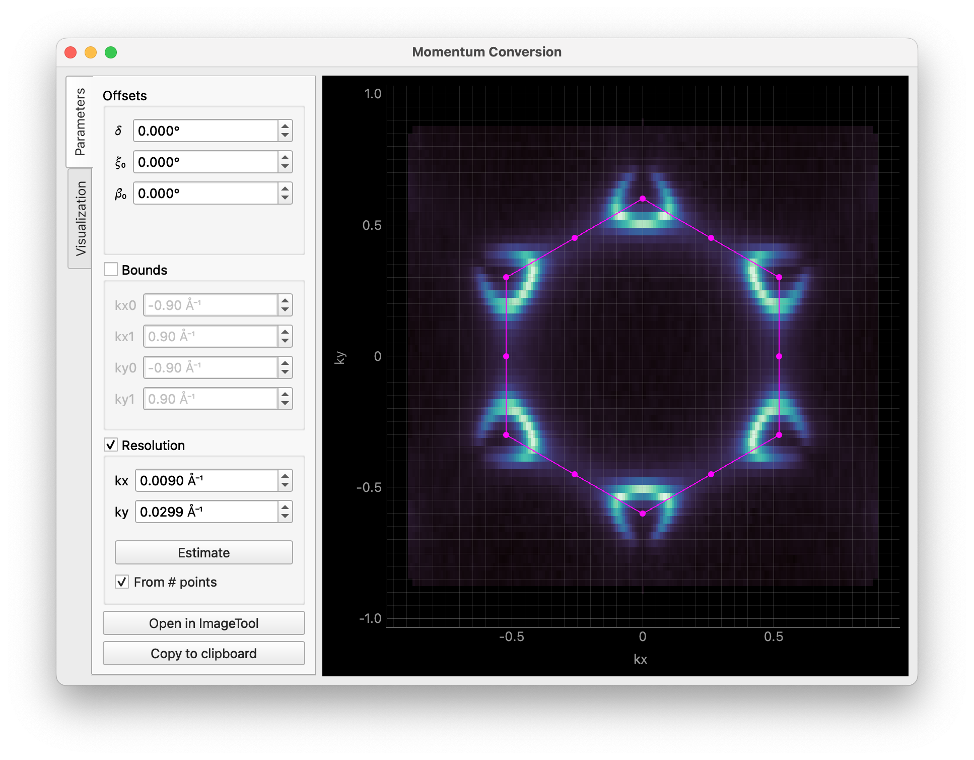
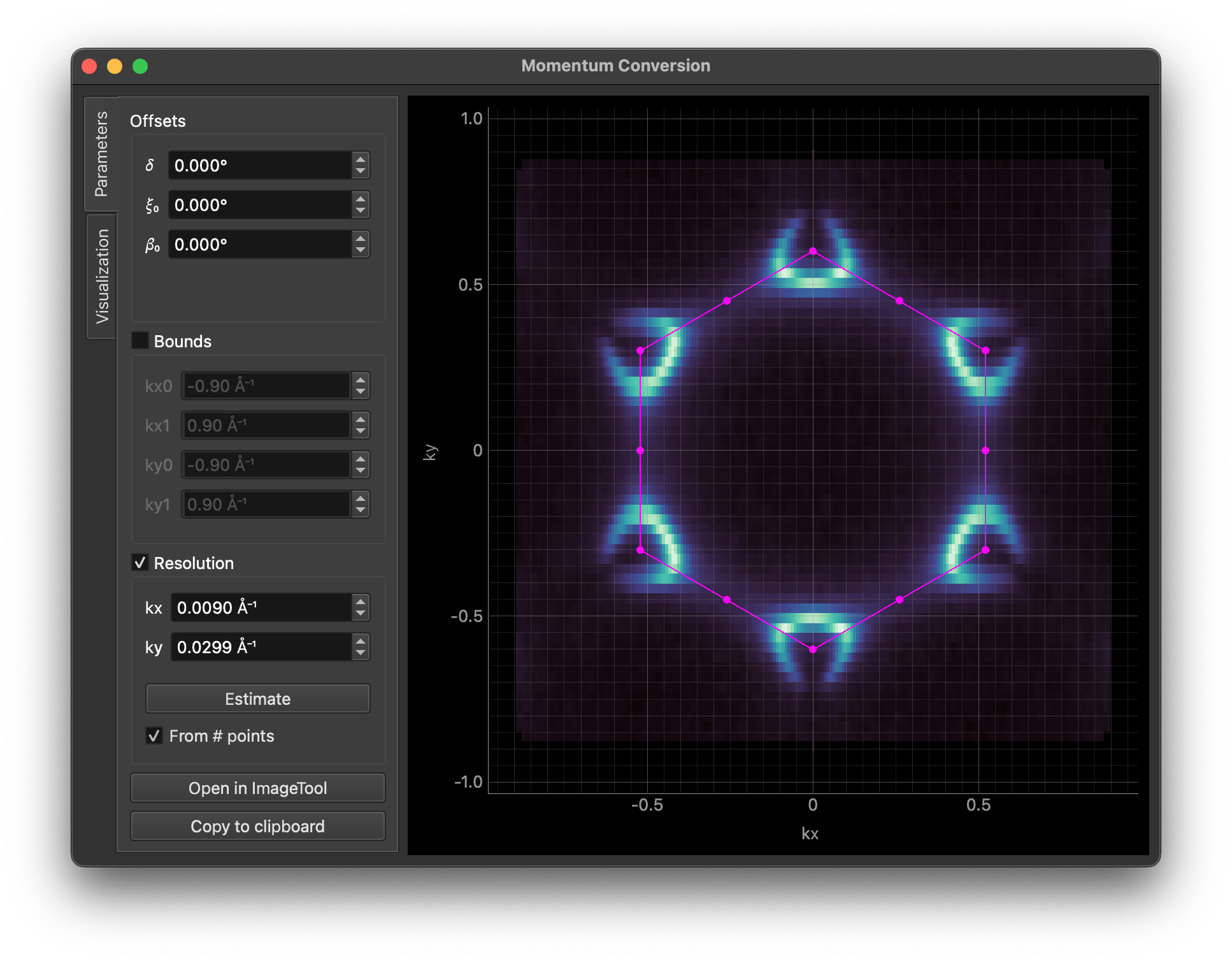
The first tab is for setting momentum conversion parameters. The image is updated in real time as you change the parameters.

Clicking Copy code will copy the code for conversion to the clipboard.

Open in ImageTool performs a full conversion and opens the result in a new ImageTool.

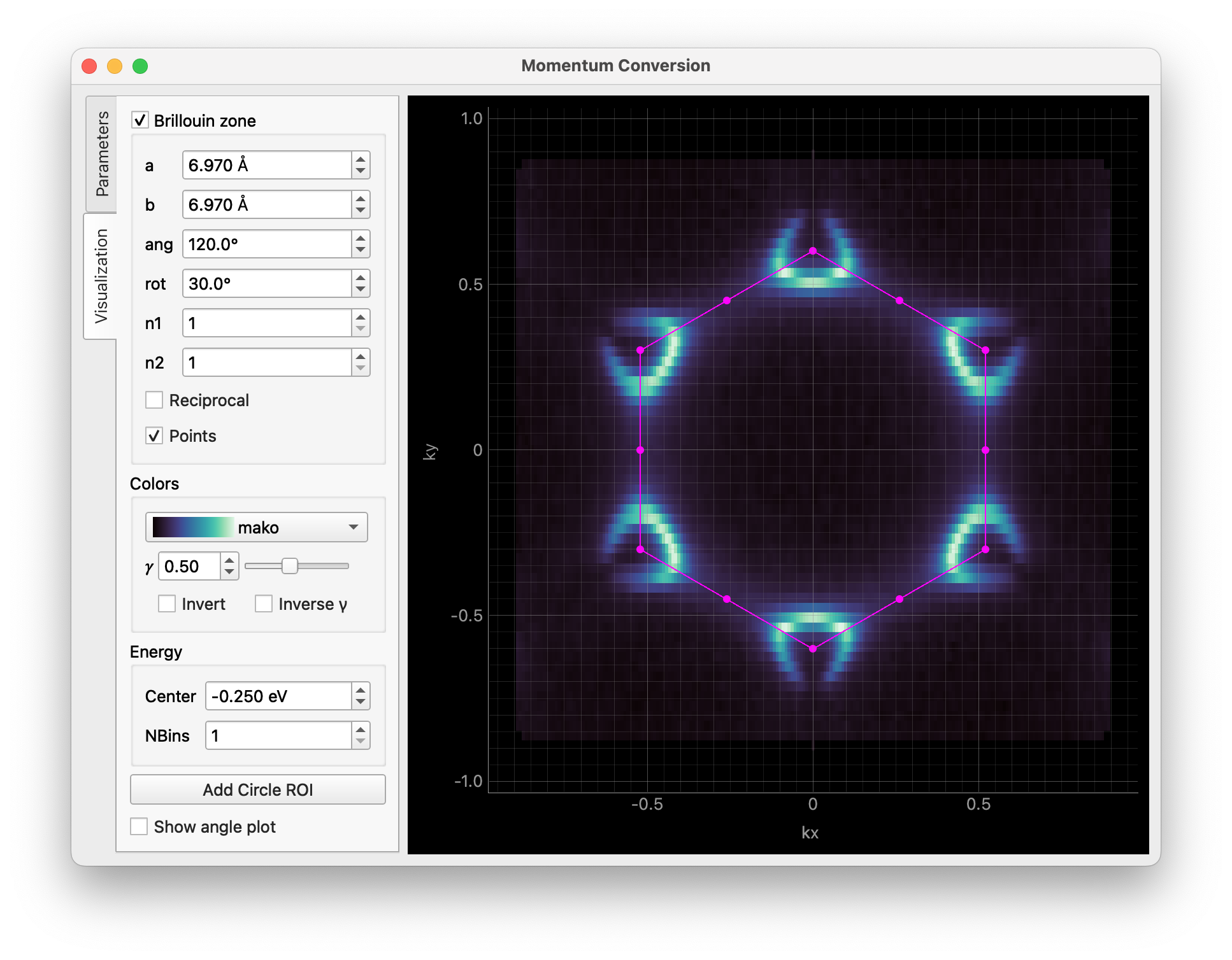
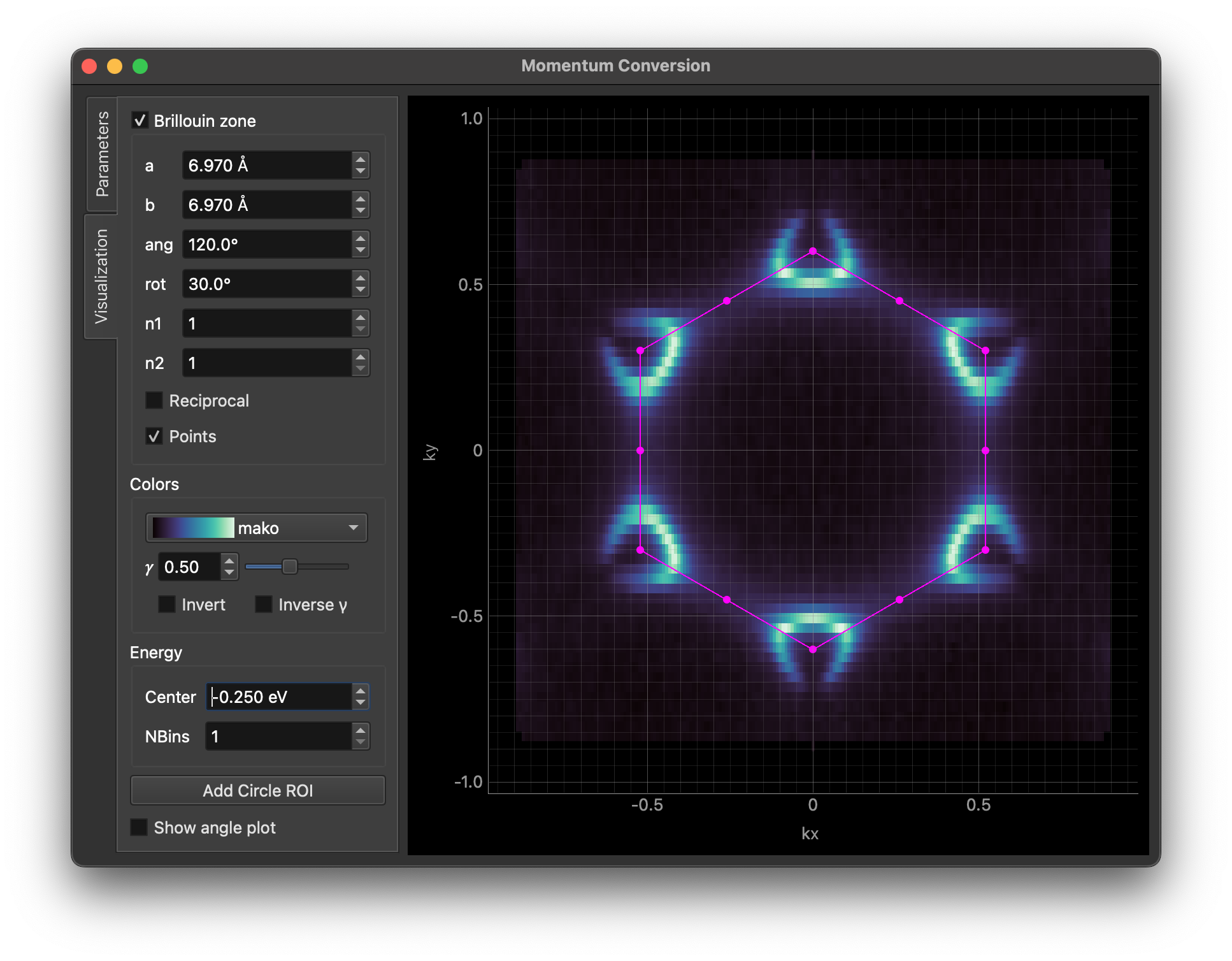
The second tab provides visualization options. You can overlay Brillouin zones and high symmetry points on the result, adjust colors, apply binning, and more.

The Add Circle ROI button allows you to add a circular region of interest to the image, which can be edited by dragging or right-clicking on it.

You can pass some parameters to customize the GUI. For example, you can set the Brillouin zone size/orientation and the colormap like this:

data.kspace.interactive(
    avec=np.array([[-3.485, 6.03], [6.97, 0.0]]), rotate_bz=30.0, cmap="viridis"
)

For all available parameters, see the documentation for erlab.interactive.ktool().

dtool¶

Interactive tool for visualizing dispersive data using derivative-based methods.

dtool can be started with erlab.interactive.dtool():

import erlab.interactive as eri

eri.dtool(data)

It can also be opened from within ImageTool from the right-click context menu of any image plot.

The %dtool line magic (see Notebook shortcuts) provides the same entry point from notebooks.

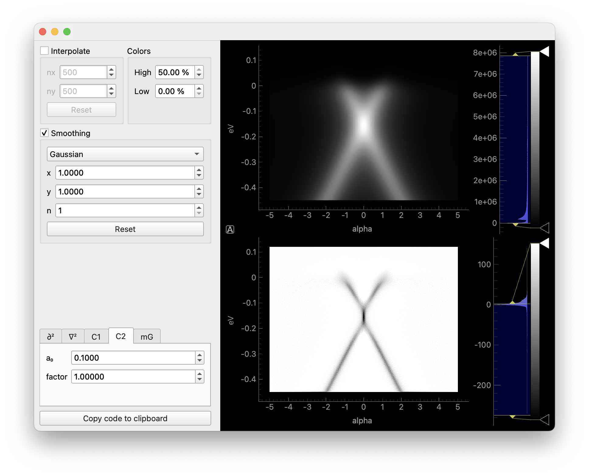
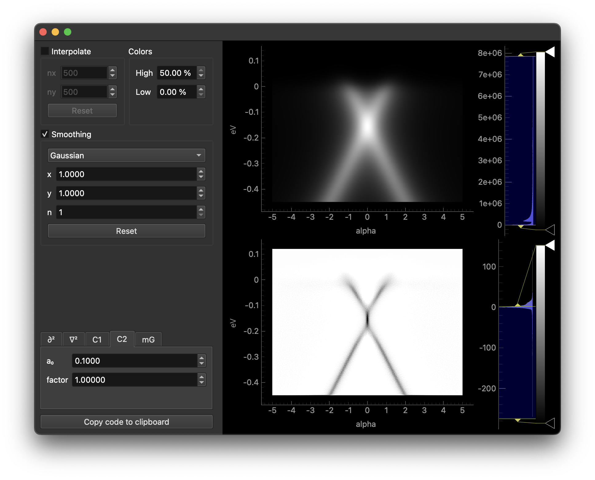
The first section interpolates the data to a grid prior to smoothing.
The second section applies smoothing prior to differentiation.
In the third section, selecting different tabs will apply different methods. Each tab contains parameters relevant to the selected method.
Clicking the copy button will copy the code for differentiation to the clipboard.
Both the smoothed data and the result can be opened in ImageTool from the right-click menu of each plot, where it can be analyzed further or saved to disk.

goldtool¶

Interactive tool for obtaining the shape of the Fermi edge (e.g., from a gold reference spectrum).

goldtool can be started with erlab.interactive.goldtool():

import erlab.interactive as eri

eri.goldtool(data)

It can also be opened from within ImageTool from the right-click context menu of any image plot.

Use the %goldtool magic (see Notebook shortcuts) to launch it directly from IPython.

ftool¶

Interactive curve-fitting tool for 1D and 2D data. By default uses erlab.analysis.fit.models.MultiPeakModel, but you can pass any 1D lmfit model.

There are three ways to start ftool.

erlab.interactive.ftool()

import erlab.interactive as eri

eri.ftool(data)

To supply a custom model:

eri.ftool(data, model=my_model)

From within ImageTool

Right-click any plot and choose ftool.
From IPython using the %ftool magic described in Notebook shortcuts.
```
%ftool data
%ftool --model my_model data
```

Overview¶

When you first open ftool, you will see a stack of controls on the left and a plot on the right, as shown below. The controls have two tabs: Setup and Fit.

Setup

Fit

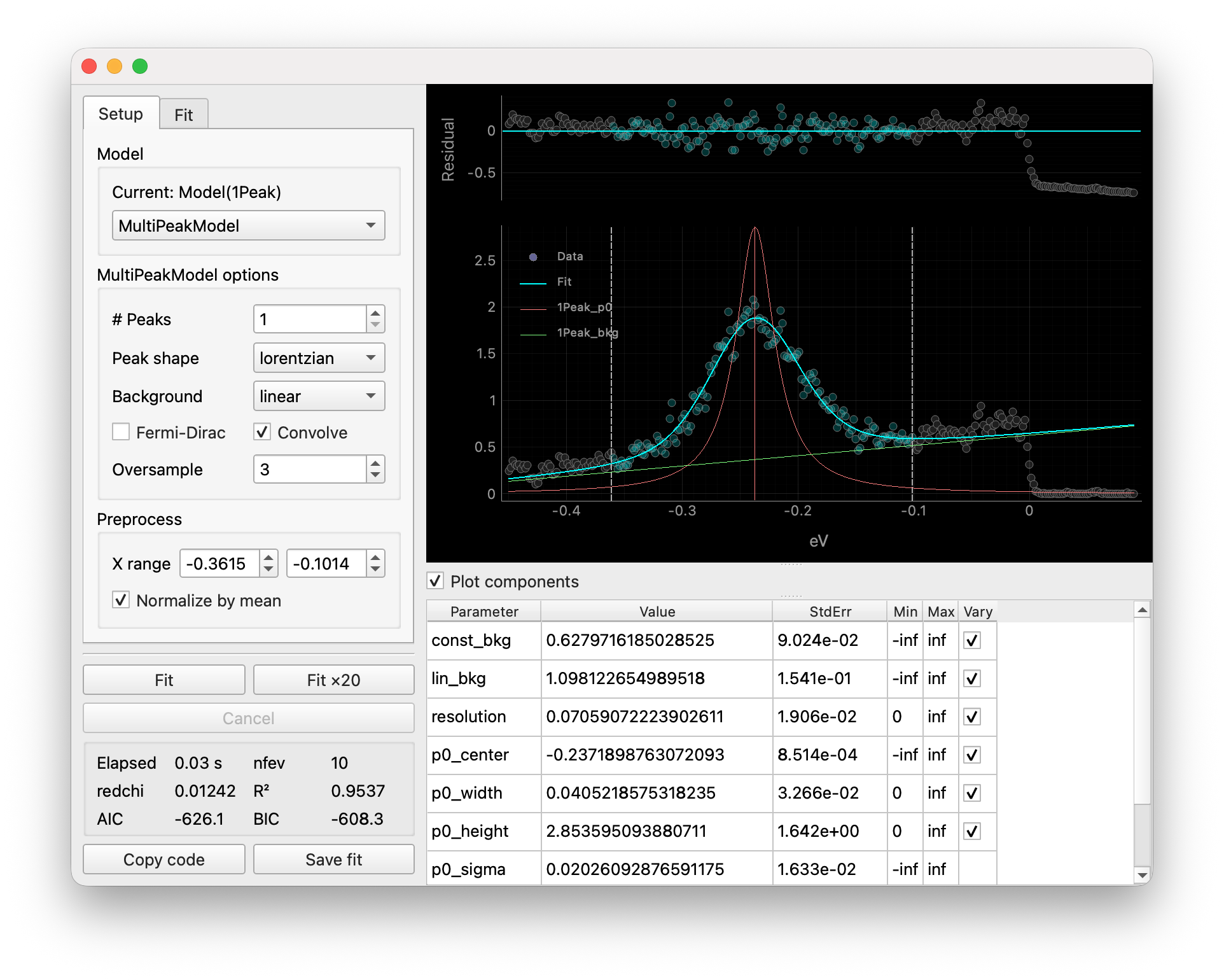
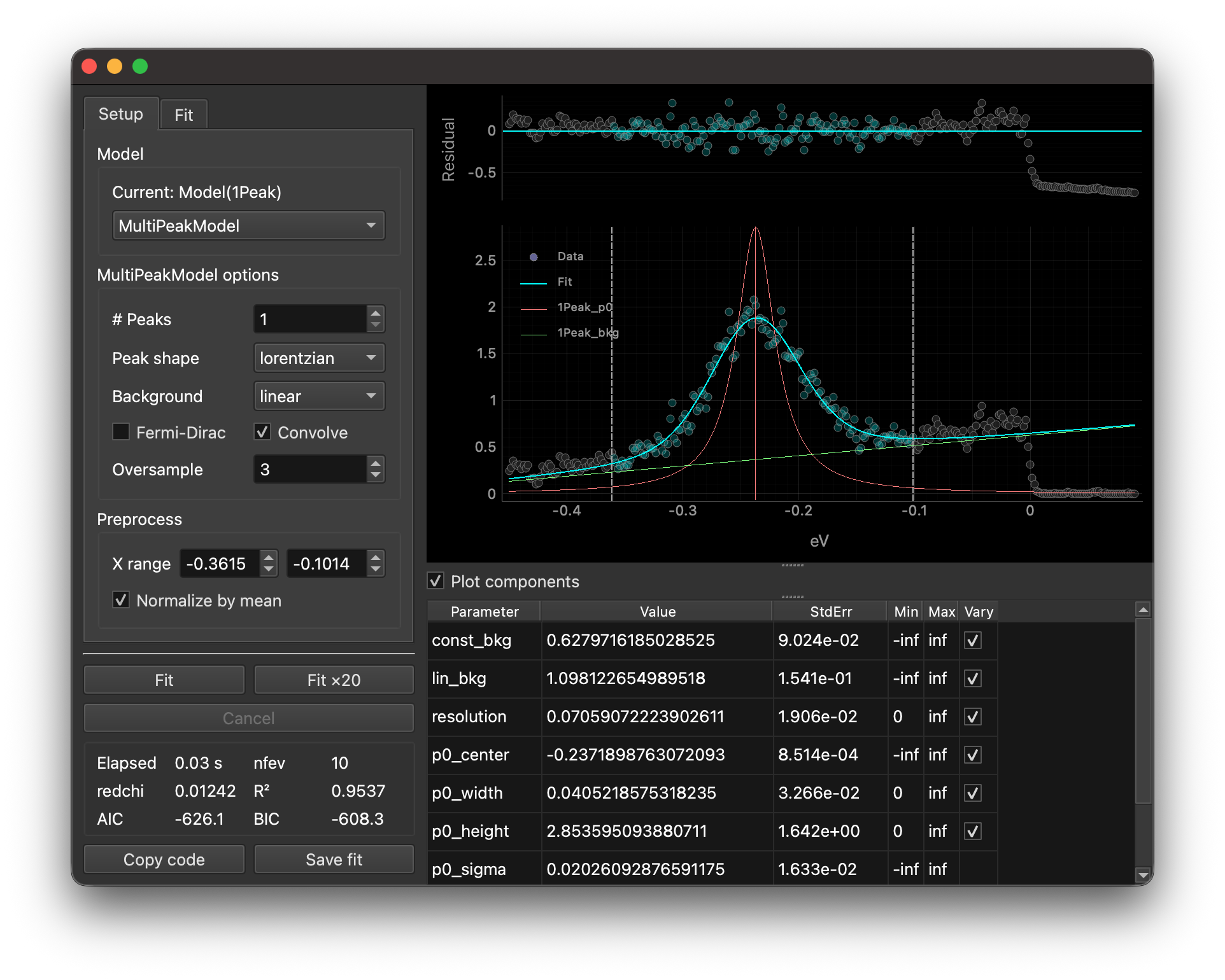
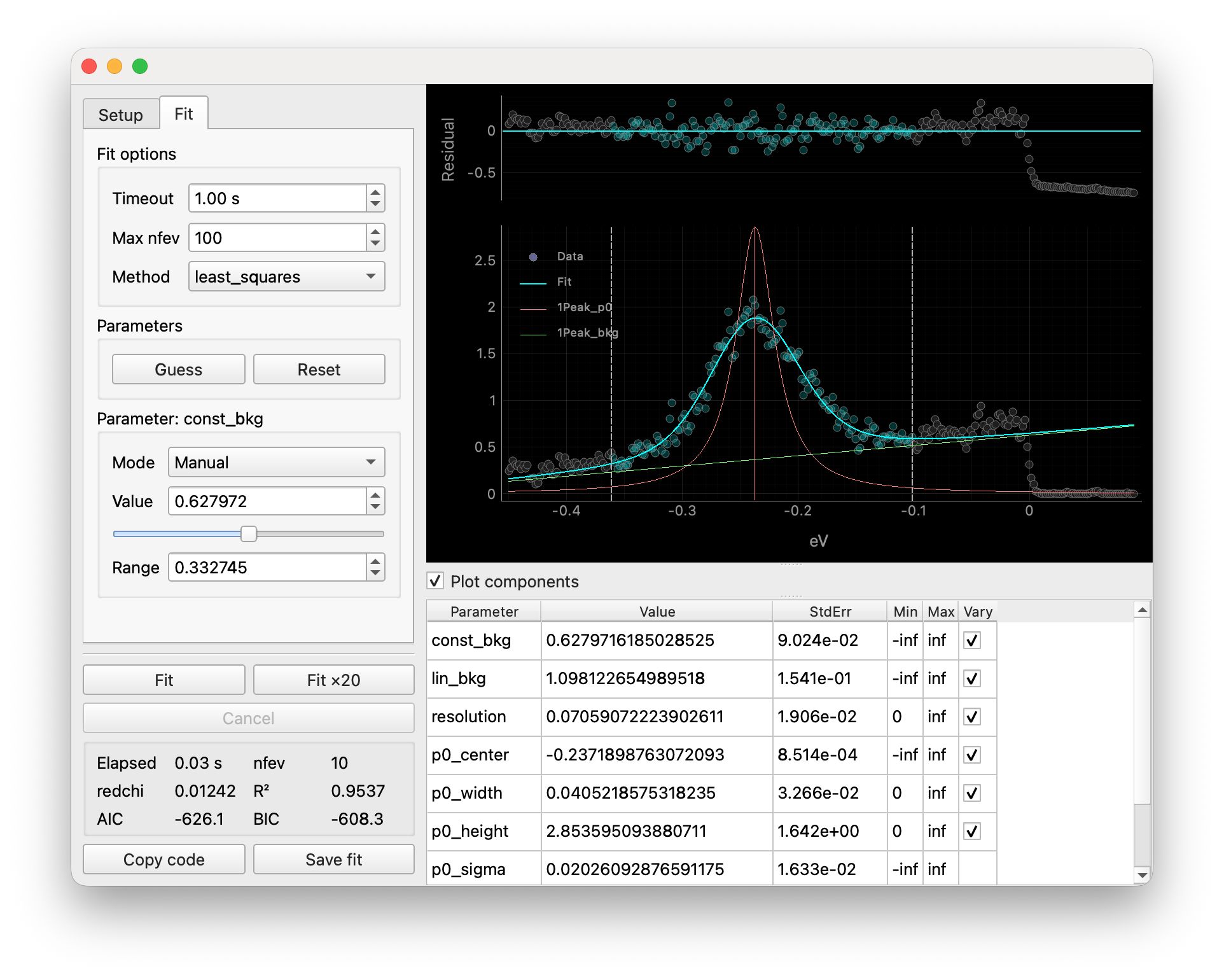
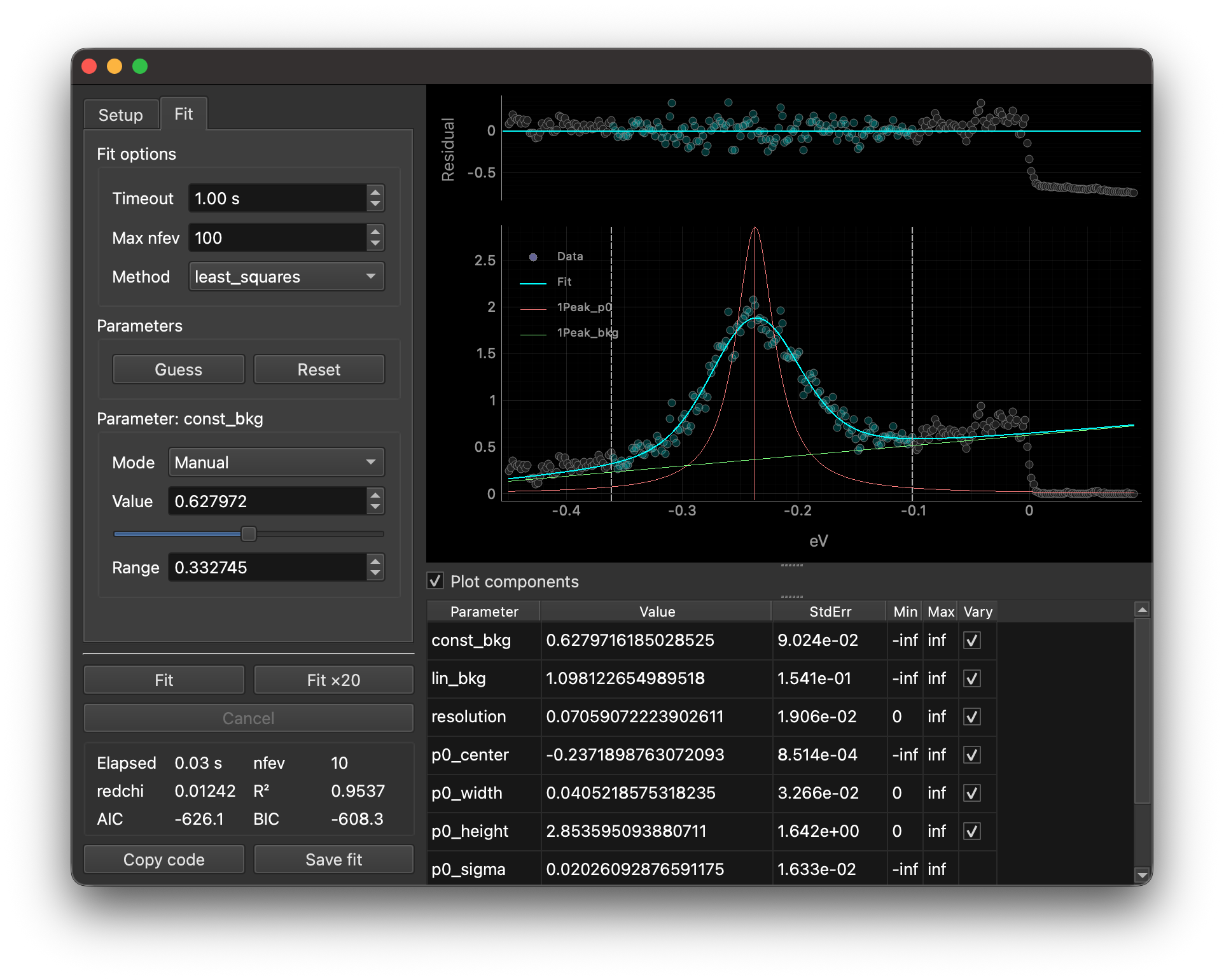
The main plot shows the data with the fit overlay, plus dashed vertical lines that define the current fit window.
- Check Plot components to show individual model components (if any). This also adds a legend for each curve. You can show/hide a component by clicking its legend entry.
The left panel contains controls for setting up and performing the fit. The Setup tab is for choosing the model and preprocessing options, while the Fit tab contains parameter settings and options related to the fitting process.

Models and options¶

First, use the Model drop-down to choose a predefined model, a user-provided model, or a model loaded from disk.

Built-in options are:
From file loads a lmfit model saved with lmfit.model.save_model().

Some models have additional options that appear below the model selector that are used to initialize the model:

MultiPeakModel:
- # Peaks and Peak shape define how many components are fit and whether they are Lorentzian or Gaussian.
- Background and Degree add a constant, linear, or polynomial background.
- Fermi-Dirac multiplies the peaks by a Fermi-Dirac distribution.
- Convolve applies instrumental broadening; Oversample controls the internal sampling density used for the convolution.
ExpressionModel:
- Edit the independent variable name in the f(...) header and type your formula in the expression box (e.g., a * x + b).
- Click Apply to rebuild the model from the current expression.
- Use Edit init script… to define helper functions or constants used in the expression.
- For more information, see the documentation for lmfit.models.ExpressionModel.

Workflow for 1D data¶

Choose your model, and set any model-specific options.
In the Preprocess group, set the fit window using X range or drag the dashed vertical bounds in the plot.

You may also choose to divide the data by its average value for better numerical stability.
Now, move on to the Fit tab.

In the Parameters group, click Guess to get initial parameters, then refine them.

You can edit parameter values, bounds, and other settings directly in the table.

You can also use the slider to adjust parameter values interactively.
Note
- Guess uses the model’s built-in guessing method (if implemented) to generate initial parameter values based on the data in the fit window. This overwrites all current parameter values.
- Any adjustment can be undone & redone with standard keyboard shortcuts.
- You can right-click parameters in the table to assign/remove expressions.
  
  For instance, to tie the position of peak 1 (p1_center) to be always 0.1 units above than peak 0 (p0_center), right-click p1_center, choose Set expression…, and enter p0_center + 0.1.
- Hover over rows in the parameter table to see tooltips with additional information.
- You can choose to fix a parameter value to be equal to a coordinate variable in the data (e.g., get the temperature from a sample_temp coordinate) by changing the Mode in the Parameter panel.
- When using MultiPeakModel, checking Plot components also shows lines at the peak centers in addition to the component curves.
  
  These lines can be dragged to quickly adjust peak positions and heights. Dragging vertically changes the height, while dragging horizontally changes the center position. Dragging vertically while holding the right mouse button changes the peak width.
Click Fit to perform the fit.

If the fit fails to converge or gives unsatisfactory results, adjust the parameters and try again.

If you want to retry automatically, use Fit×20. You can increase Max nfev in the Fit options group, which sets the maximum number of function evaluations allowed. The nfev stat is highlighted in red when the fit hits this limit without converging.

About Fit ×20

Fit ×20 performs a sequence of 20 fits on the same data. After each run, the fitted parameters are fed back in as the initial parameters for the next run. This can help in nonlinear or highly correlated models where a single fit gets close but not fully converged. Reusing the previous best-fit parameters often nudges the optimizer into a better solution without you having to manually tweak values between runs.
Use Copy code to copy the reproducible code for this fit to the clipboard, or use Save fit to save the results with xarray_lmfit.save_fit().

Workflow for 2D data¶

For 2D data, an additional image and a parameter-versus-coordinate plot are shown, along with a Transpose button and index navigation controls.

Setup

Fit

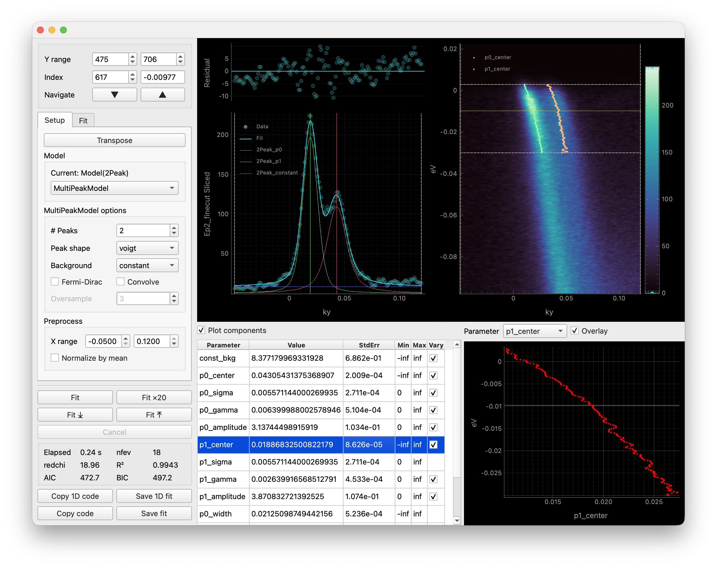
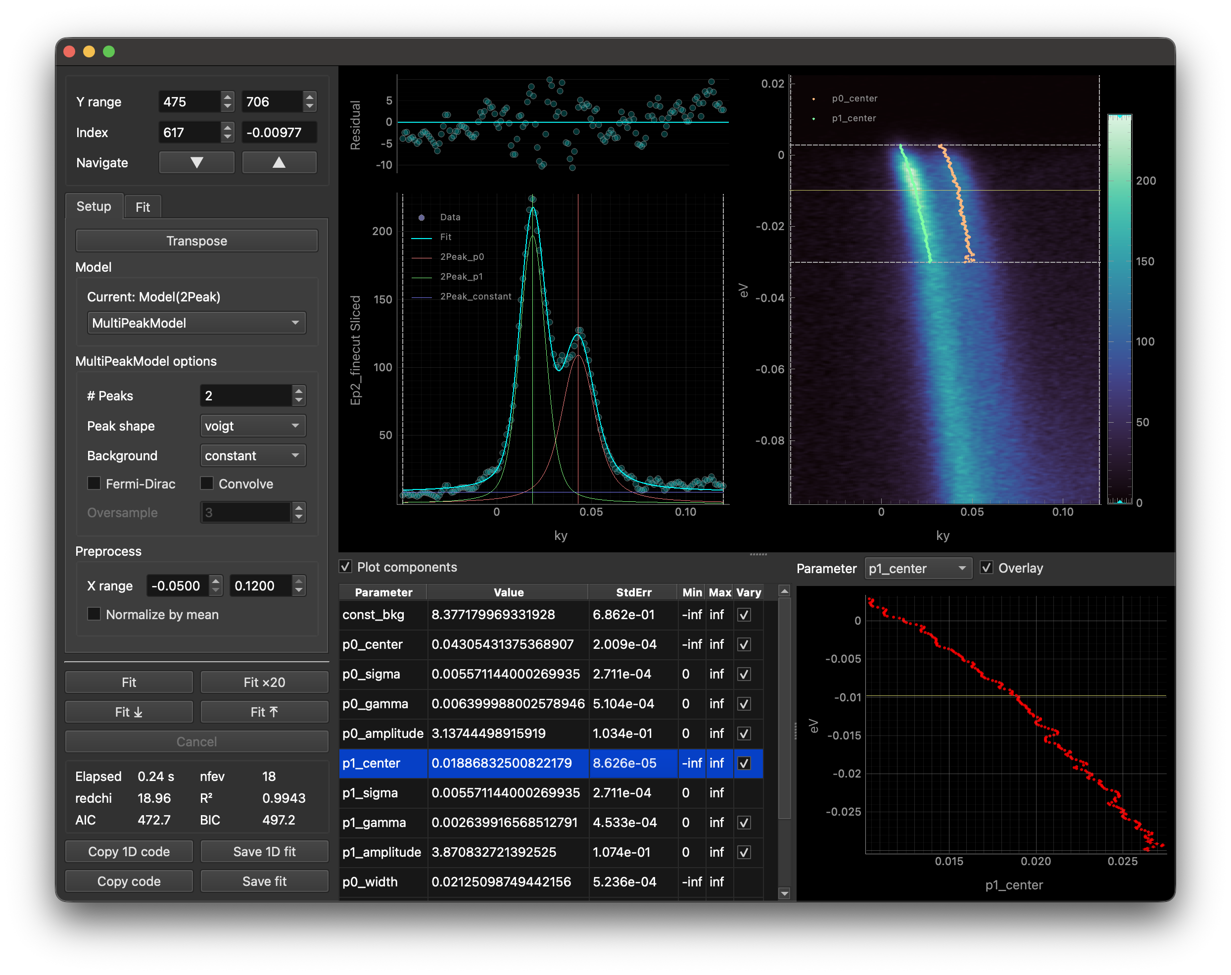
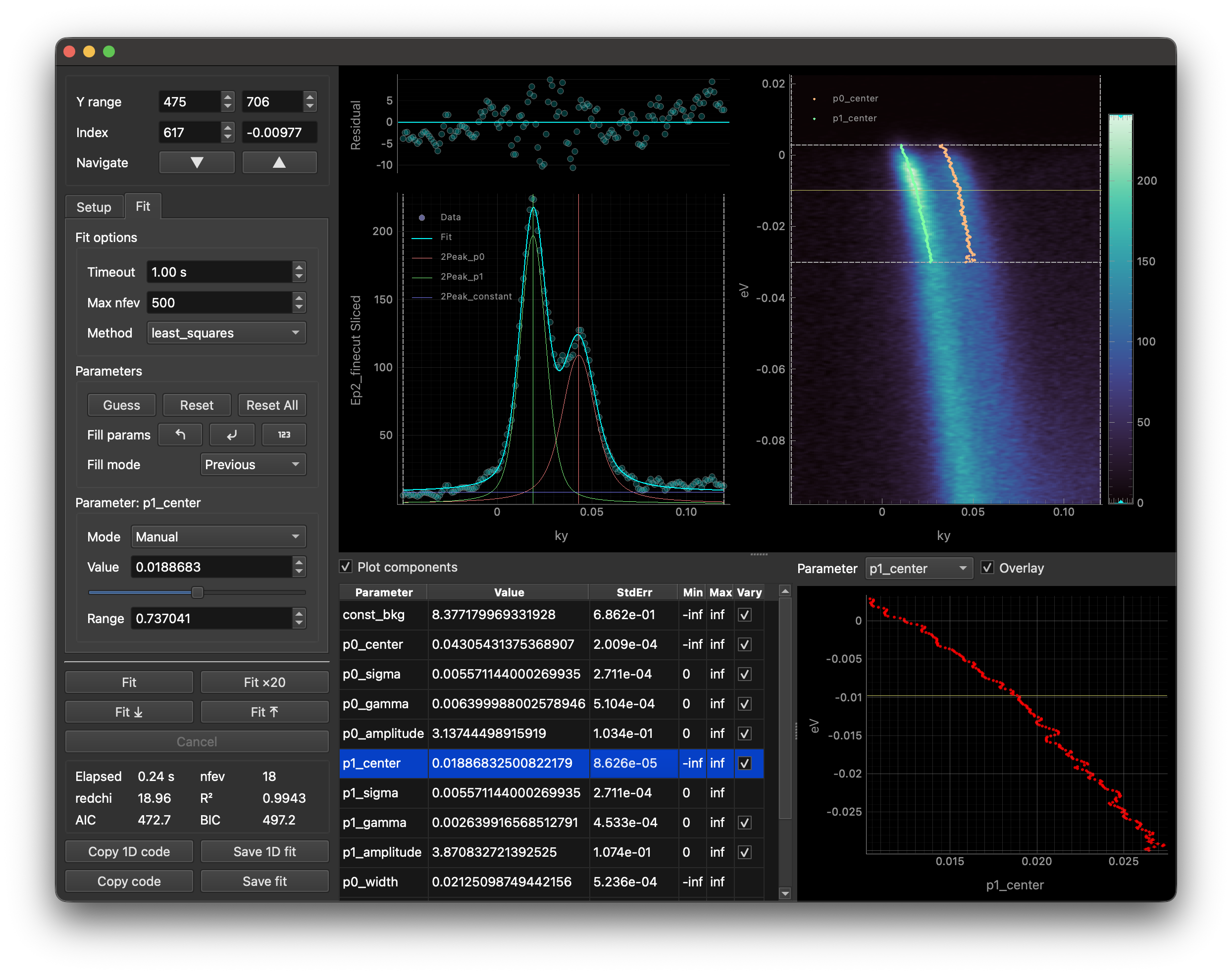
For 2D data, the tool fits a stack of 1D curves.

Check if the data dimensions are in the correct order. The axis you wish to sweep along is the vertical axis; if the image is rotated 90 degrees from what you expect, click Transpose to swap the axes.
Set the X window with X range or by dragging the vertical dashed lines.
Choose the Y range to fit: use the Y range spin boxes or drag the horizontal dashed lines in the image.
Pick a representative Y index with Index (or drag the yellow cursor), then tune the fit parameters for that slice like in the 1D workflow above. Once you are satisfied with the fit, proceed to the next step.
Decide how parameters propagate between EDCs using Fill mode.
- Previous keeps the last good parameters.
- Extrapolate linearly projects parameters from the previous two slices.
- Use None when all slices already have reasonable initial parameters, and you just want to fit them all without parameter propagation.
Start the 2D sequence with Fit ⤒ or Fit ⤓. The tool will step through the selected range while populating the parameters according to the chosen mode.
Inspect the parameter plot to verify trends. If a slice fails, move to it with Index, fix the parameters, then continue the sequence.
When all indices in the range are fitted, click Save fit to export the combined results or Copy code to generate reproducible code for the full 2D fit. These buttons are only enabled after the full sequence is complete.

Reopening saved fits¶

You can reopen a saved fit by loading the dataset with xarray_lmfit.load_fit() and passing it directly to erlab.interactive.ftool().

Saved fits restore the stored data, the serialized model (when available), and the fitted parameter values. For 2D fits, all slices must share the same model definition.

Note

The data is cropped to the fit range used during saving, so reopening a saved fit will only show the data within the original fit window. To preserve the full data, open ftool from data in the ImageTool manager and save as a workspace.

restool¶

Interactive tool for fitting a single resolution-broadened Fermi-Dirac distribution to an energy distribution curve (EDC). The momentum range to be integrated over can be adjusted interactively. This is useful for quickly determining the energy resolution of the current experiment.

The GUI can be invoked with erlab.interactive.restool():

import erlab.interactive as eri

eri.restool(data)

It can also be opened from within ImageTool from the right-click context menu of any image plot that contains an energy axis.

The %restool magic (see Notebook shortcuts) provides a quick way to launch it from IPython.

meshtool¶

Interactive tool for removing grid-like mesh artifacts from fixed mode ARPES data.

The GUI can be invoked with erlab.interactive.meshtool():

import erlab.interactive as eri

eri.meshtool(data)

It can also be opened from within ImageTool by clicking View → Open in meshtool.

The %meshtool magic (see Notebook shortcuts) provides a quick way to launch it from IPython.

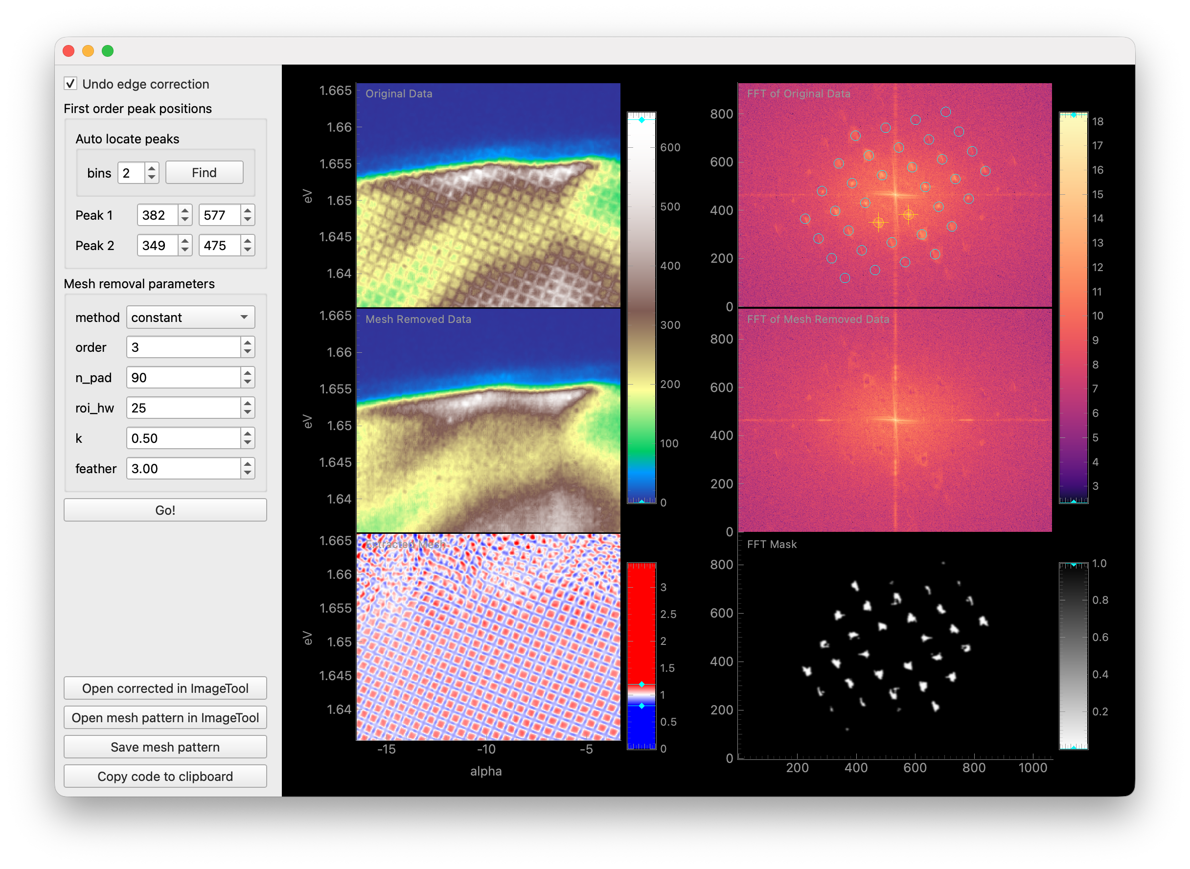
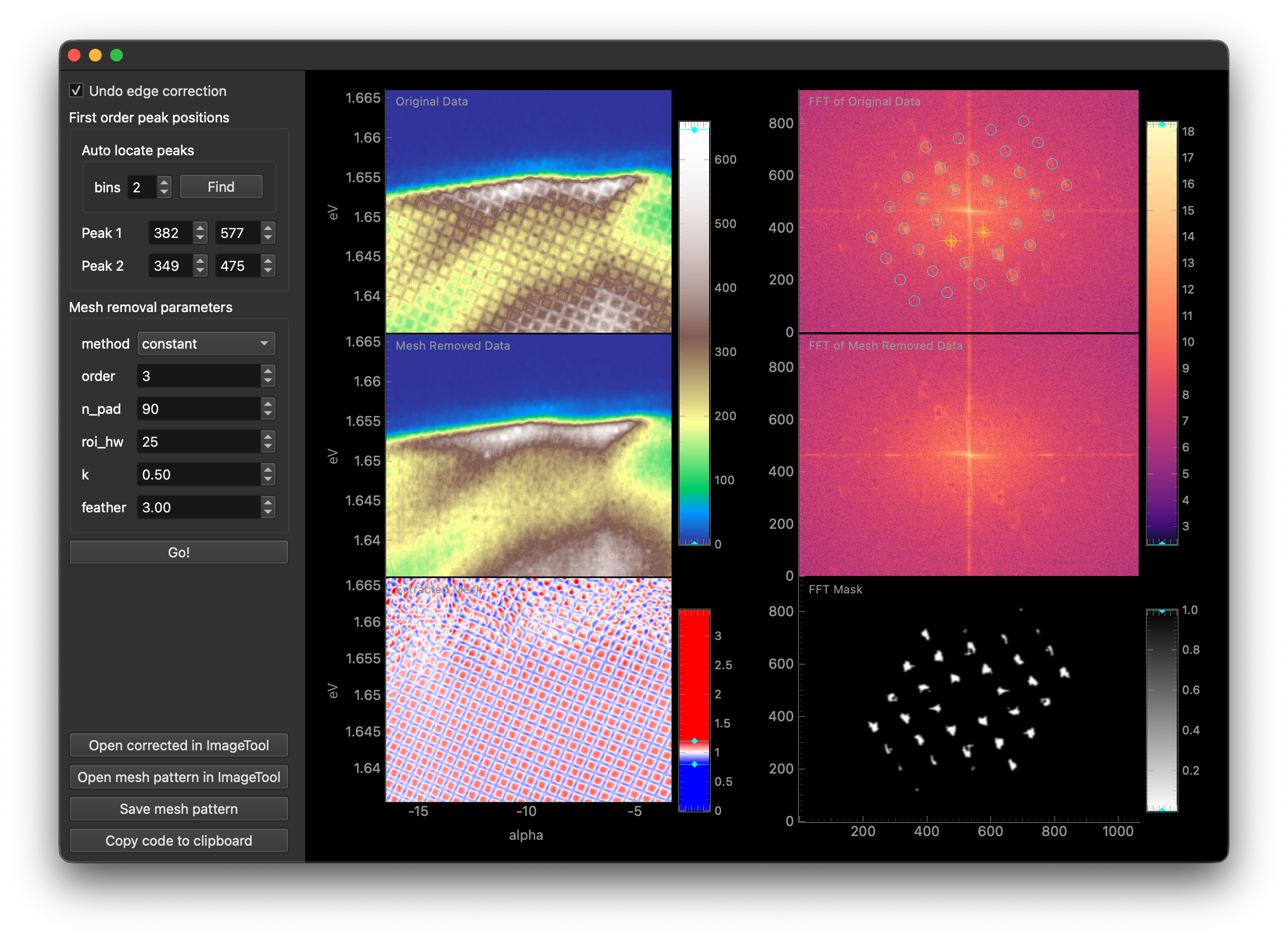
This tool accepts any DataArray with eV and alpha dimensions. When additional dimensions are present, the data will be averaged over those dimensions to detect the mesh pattern. The original data will be corrected using the detected mesh parameters.

The first checkbox enables/disables undoing of software edge correction for straight analyzer slits that some analyzers apply automatically (currently only tested with Scienta DA30L).
In the next section, you must specify the location of the first order mesh peaks in the FFT of the data.
- Drag the two yellow targets on the FFT plot over the two first order mesh peaks by dragging them with the mouse.
- Alternatively, an automatic search can be performed by clicking Find under Auto locate peaks.
In the final section, several parameters for mesh removal are provided. For more information on these parameters, see the documentation for erlab.analysis.mesh.remove_mesh(). You may have to experiment with these parameters to achieve optimal results for your dataset.
Once you are satisfied with the parameters, click Go! to perform mesh removal.

Note

Mesh removal is currently experimental and may not work well for all datasets, and may introduce unwanted artifacts. Please use with caution and verify the results carefully.

Data explorer¶

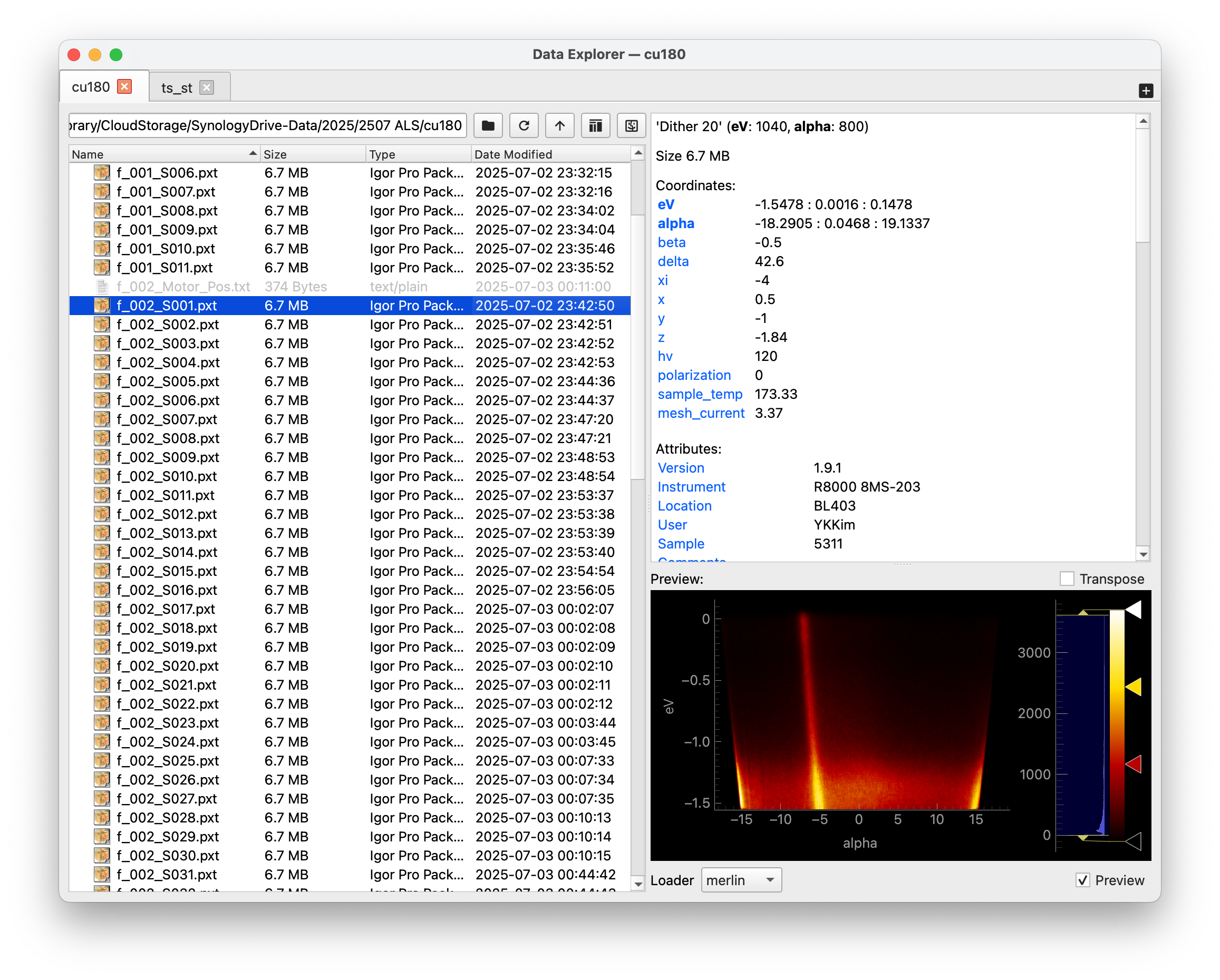
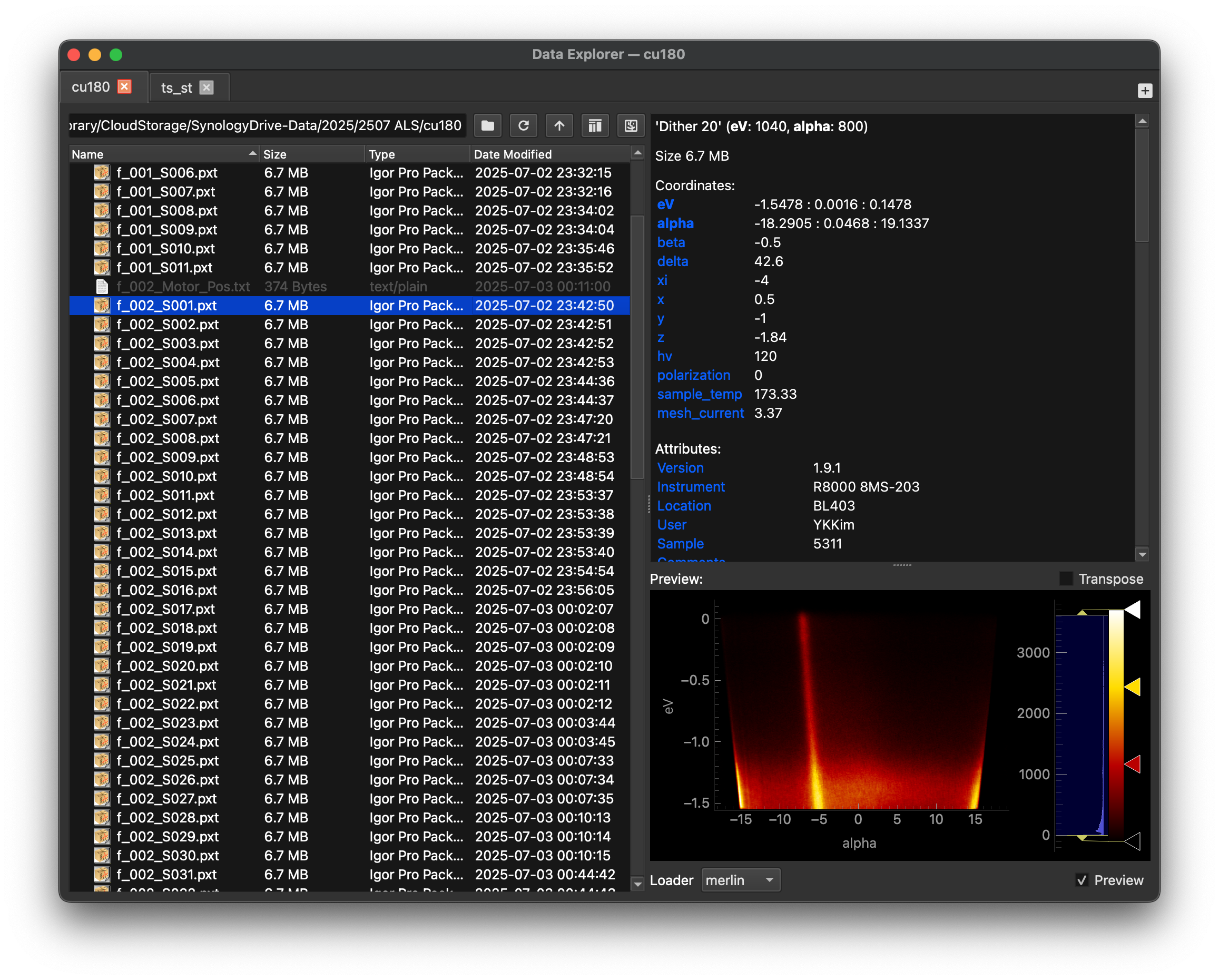
Provides a file-browser-like interface for exploring and visualizing ARPES data stored on your disk. See erlab.interactive.data_explorer() for more information.

BZPlotter¶

This tool is not an analysis tool, but rather a utility for creating plots of three-dimensional Brillouin zones and exporting them as vector graphics.

The GUI can be invoked with erlab.interactive.bzplot.BZPlotter:

import erlab.interactive as eri

eri.bzplot.BZPlotter()

Once opened, a matplotlib figure window will appear alongside a control panel for adjusting the lattice parameters. The figure can be rotated interactively using the mouse, and the plot can be exported as any of the formats supported by matplotlib via the standard matplotlib save button.

Notebook shortcuts¶

Loading the erlab.interactive IPython extension (%load_ext erlab.interactive) registers convenient line magics for quickly launching the various interactive tools from within a Jupyter notebook or IPython console.

%ktool --cmap viridis darr.sel(eV=0)

%dtool darr

%goldtool darr.isel(beta=1)

%restool darr.mean(dim='kx')

%ftool --model my_model darr