Momentum conversion
Momentum conversion in ERLabPy is exact with no small angle approximation, but is also very fast, thanks to the numba-accelerated trilinear interpolation in erlab.analysis.interpolate.
Nomenclature
Momentum conversion in ERLabPy follows the nomenclature from Ishida and Shin [3].
All experimental geometry can be classified into two configurations, Type 1 and Type 2, based on the relative position of the rotation axis and the analyzer slit. These can be further divided into 4 configurations depending on the use of photoelectron deflectors (DA).
Definition of angles differ for each geometry, but in all cases, \(\delta\) is the azimuthal angle that indicates in-plane rotation, \(\alpha\) is the angle detected by the analyzer, and \(\beta\) is the angle along which mapping is performed.
For instance, imagine a typical Type 1 setup with a vertical slit that acquires maps by rotating about the z axis in the lab frame. In this case, the polar angle (rotation about z) is \(\beta\), and the tilt angle becomes \(\xi\).
The following table summarizes angle conventions for commonly encountered configurations.
Analyzer slit orientation |
Mapping angle |
Configuration |
Polar |
Tilt |
Deflector |
Azimuth |
Analyzer |
|---|---|---|---|---|---|---|---|
Vertical |
Polar |
1 (Type 1) |
|
|
|
|
|
Horizontal |
Tilt |
2 (Type 2) |
|
|
|||
Vertical |
Deflector |
3 (Type 1 + DA) |
|
|
|
||
Horizontal |
4 (Type 2 + DA) |
Note
Analyzers that can measure two-dimensional angular information simultaneously (e.g. time-of-flight analyzers) can be treated like hemispherical analyzers equipped with a deflector.
import matplotlib.pyplot as plt
import numpy as np

import erlab.plotting as eplt
Momentum conversion
Note
For momentum conversion to work properly, the data must follow the conventions listed here.
Setting parameters
Parameters that are needed for momentum conversion are:
The information about the experimental configuration
Work function of the system
The inner potential \(V_0\) (for photon energy dependent data)
Angle offsets
These parameters are all stored as data attributes. The kspace accessor provides various ways to access and modify these parameters.
Experimental configuration
The first step is to set the experimental configuration. Most of the time, this information is already recorded in the data file by the data loader plugin. If not, it can be set manually using xarray.DataArray.kspace.configuration:
data.kspace.configuration = erlab.constants.AxesConfiguration.Type1DA
This will set the configuration to Type 1 with a deflector. The configuration can also be set using numbers:
data.kspace.configuration = 3
Sometimes, the automatically determined configuration may be incorrect. For example, plugins for setups equipped with an electrostatic deflector will assign configuration 3 or 4 to the data, but the data may have been acquired without the deflector, in which case configuration 1 or 2 should be used. Also, some setups (e.g. ALS BL7) have variable slit orientation by allowing the analyzer to be rotated about the lens axis. As such, it is not always possible to determine the configuration from the data alone. In these cases, the configuration can be converted with xarray.DataArray.kspace.as_configuration() which takes a configuration number or an enum as an argument. For example, consider a data taken at ALS BL7 with configuration 2 (horizontal slit, tilt map). By default, the loader will assign configuration 3 (vertical slit, DA map) to the data, which is incorrect. To convert the data to configuration 2, you can do:
data = data.kspace.as_configuration(2)
which returns a copy of the data with the configuration set to 2, and the coordinates renamed accordingly.
Note
The method assumes a typical ARPES setup with a vertical cryostat. For complex setups, the user should manually set the configuration attribute and rename the coordinates.
Work function of the system
The work function of the system can be set using xarray.DataArray.kspace.work_function:
data.kspace.work_function = 4.5
Inner potential \(V_0\)
The inner potential (for photon energy dependent data) can be set using xarray.DataArray.kspace.inner_potential:
data.kspace.inner_potential = 10.0
Angle offsets
Angle offsets can be set using xarray.DataArray.kspace.offsets. For demonstration, let’s generate some example data, this time in angle coordinates.
from erlab.io.exampledata import generate_data_angles

dat = generate_data_angles(shape=(200, 60, 300), assign_attributes=True, seed=1).T
dat
<xarray.DataArray (eV: 300, beta: 60, alpha: 200)> Size: 29MB
129.6 115.6 96.64 76.55 65.6 56.97 ... 0.1651 0.004688 0.1373 0.5505 0.1394
Coordinates:
  * alpha    (alpha) float64 2kB -15.0 -14.85 -14.7 -14.55 ... 14.7 14.85 15.0
  * beta     (beta) float64 480B -15.0 -14.49 -13.98 -13.47 ... 13.98 14.49 15.0
  * eV       (eV) float64 2kB -0.45 -0.4481 -0.4462 ... 0.1162 0.1181 0.12
    xi       float64 8B 0.0
    delta    float64 8B 0.0
    hv       float64 8B 50.0
Attributes:
    configuration:        1
    sample_temp:          20.0
sample_workfunction: 4.5To view the currently set angle offsets:
dat.kspace.offsets
| delta | 0.0 |
|---|---|
| xi | 0.0 |
| beta | 0.0 |
Since we haven’t set any offsets, they are all zero. Now, if we want to set the azimuthal angle to 60 degrees and the polar offset to 30 degrees, we can update the offsets as follows:
dat.kspace.offsets.update(delta=60.0, beta=30.0)
| delta | 60.0 |
|---|---|
| xi | 0.0 |
| beta | 30.0 |
The offsets behave like a dictionary, and you can also reset or override all offsets at once using a dictionary:
dat.kspace.offsets = dict(delta=30.0)

dat.kspace.offsets
| delta | 30.0 |
|---|---|
| xi | 0.0 |
| beta | 0.0 |
See xarray.DataArray.kspace.offsets for more ways to access and modify offsets.
Note
Offsets can be easily determined with the interactive momentum conversion tool.
Converting to momentum space
Momentum conversion is done by the xarray.DataArray.kspace.convert() method after applying appropriate offsets. The bounds and resolution are automatically determined from the data if no input is provided. The method returns a new DataArray in momentum space.
dat.kspace.offsets = dict(delta=30, xi=0.0, beta=0.0)
dat.kspace.work_function = 4.5

dat_kconv = dat.kspace.convert()
dat_kconv
<xarray.DataArray (kx: 418, ky: 414, eV: 300)> Size: 415MB
nan nan nan nan nan nan nan nan nan nan ... nan nan nan nan nan nan nan nan nan
Coordinates:
    xi       float64 8B 0.0
    delta    float64 8B 0.0
    hv       float64 8B 50.0
  * kx       (kx) float64 3kB -1.208 -1.202 -1.197 -1.191 ... 1.197 1.202 1.208
  * ky       (ky) float64 3kB -1.197 -1.191 -1.185 -1.18 ... 1.185 1.191 1.197
  * eV       (eV) float64 2kB -0.45 -0.4481 -0.4462 ... 0.1162 0.1181 0.12
Attributes:
    configuration:        1
    sample_temp:          20.0
    sample_workfunction:  4.5
    delta_offset:         30.0
    xi_offset:            0.0
beta_offset: 0.0Let us plot the original and converted data side by side.
fig, axs = plt.subplots(1, 2, layout="compressed")
eplt.plot_array(dat.qsel(eV=-0.3), ax=axs[0], aspect="equal")
eplt.plot_array(dat_kconv.qsel(eV=-0.3), ax=axs[1], aspect="equal")
<matplotlib.image.AxesImage at 0x797ec2c97890>

We can see the effect of angle offsets on the conversion.
The step size and bounds of momentum coordinates can be set manually as well:
dat_kconv = dat.kspace.convert(
    bounds=dict(kx=(-0.5, 0.5), ky=(-0.5, 0.5)),
    resolution=dict(kx=0.01, ky=0.01),
)
dat_kconv
<xarray.DataArray (kx: 101, ky: 101, eV: 300)> Size: 24MB
450.3 430.5 410.3 412.9 403.1 380.8 ... 0.06322 0.01239 0.05766 0.09326 0.1791
Coordinates:
    xi       float64 8B 0.0
    delta    float64 8B 0.0
    hv       float64 8B 50.0
  * kx       (kx) float64 808B -0.5 -0.49 -0.48 -0.47 ... 0.47 0.48 0.49 0.5
  * ky       (ky) float64 808B -0.5 -0.49 -0.48 -0.47 ... 0.47 0.48 0.49 0.5
  * eV       (eV) float64 2kB -0.45 -0.4481 -0.4462 ... 0.1162 0.1181 0.12
Attributes:
    configuration:        1
    sample_temp:          20.0
    sample_workfunction:  4.5
    delta_offset:         30.0
    xi_offset:            0.0
beta_offset: 0.0fig, axs = plt.subplots(1, 2, layout="compressed")
eplt.plot_array(dat.qsel(eV=-0.3), ax=axs[0], aspect="equal")
eplt.plot_array(dat_kconv.qsel(eV=-0.3), ax=axs[1], aspect="equal")
<matplotlib.image.AxesImage at 0x797ec10002d0>

The target momentum coordinates can also be set manually:
dat.kspace.convert(kx=np.linspace(-0.6, 0.6, 100))
<xarray.DataArray (kx: 100, ky: 414, eV: 300)> Size: 99MB
nan nan nan nan nan nan nan nan nan nan ... nan nan nan nan nan nan nan nan nan
Coordinates:
    xi       float64 8B 0.0
    delta    float64 8B 0.0
    hv       float64 8B 50.0
  * kx       (kx) float64 800B -0.6 -0.5879 -0.5758 ... 0.5758 0.5879 0.6
  * ky       (ky) float64 3kB -1.197 -1.191 -1.185 -1.18 ... 1.185 1.191 1.197
  * eV       (eV) float64 2kB -0.45 -0.4481 -0.4462 ... 0.1162 0.1181 0.12
Attributes:
    configuration:        1
    sample_temp:          20.0
    sample_workfunction:  4.5
    delta_offset:         30.0
    xi_offset:            0.0
beta_offset: 0.0Converting coordinates only
Sometimes, we need to obtain the converted coordinates in momentum space without modifying the data grid.
This can be done using xarray.DataArray.kspace.convert_coords() which adds momentum coordinates to the DataArray.
The code below demonstrates a possible use case where we convert the coordinates of a cut to momentum space and overlay the location of the cut on the converted constant energy map.
First, we select a cut from the original data along constant beta.
cut = dat.qsel(beta=-10)
cut
<xarray.DataArray (eV: 300, alpha: 200)> Size: 480kB
171.5 221.9 379.4 661.3 1.126e+03 ... 8.253e-07 0.000433 0.02783 0.112 0.03038
Coordinates:
  * eV       (eV) float64 2kB -0.45 -0.4481 -0.4462 ... 0.1162 0.1181 0.12
  * alpha    (alpha) float64 2kB -15.0 -14.85 -14.7 -14.55 ... 14.7 14.85 15.0
    beta     float64 8B -9.915
    xi       float64 8B 0.0
    delta    float64 8B 0.0
    hv       float64 8B 50.0
Attributes:
    configuration:        1
    sample_temp:          20.0
    sample_workfunction:  4.5
    delta_offset:         30.0
    xi_offset:            0.0
beta_offset: 0.0cut = cut.kspace.convert_coords()
cut
<xarray.DataArray (eV: 300, alpha: 200)> Size: 480kB
171.5 221.9 379.4 661.3 1.126e+03 ... 8.253e-07 0.000433 0.02783 0.112 0.03038
Coordinates:
  * eV       (eV) float64 2kB -0.45 -0.4481 -0.4462 ... 0.1162 0.1181 0.12
  * alpha    (alpha) float64 2kB -15.0 -14.85 -14.7 -14.55 ... 14.7 14.85 15.0
    beta     float64 8B -9.915
    xi       float64 8B 0.0
    delta    float64 8B 0.0
    hv       float64 8B 50.0
    kx       (eV, alpha) float64 480kB 0.4848 0.477 0.4692 ... -1.056 -1.063
    ky       (eV, alpha) float64 480kB 0.9403 0.9363 0.9322 ... 0.05538 0.05063
Attributes:
    configuration:        1
    sample_temp:          20.0
    sample_workfunction:  4.5
    delta_offset:         30.0
    xi_offset:            0.0
beta_offset: 0.0We can see that coordinate conversion adds momentum coordinates kx and ky, but does not affect any existing coordinates. Now, let’s annotate the cut location on the constant energy map.
fig, ax = plt.subplots()

dat.kspace.convert().qsel(eV=-0.3).qplot(ax=ax, aspect="equal")

mdc = cut.qsel(eV=-0.3)
ax.plot(mdc.ky, mdc.kx, color="r")
[<matplotlib.lines.Line2D at 0x797ec10d2ad0>]

\(k_z\)-dependent data
Converting \(k_z\)-dependent data can be done in the exact same way by choosing an appropriate value for the inner potential \(V_0\). Let’s generate some example data that resembles photon energy dependent cuts.
from erlab.io.exampledata import generate_hvdep_cuts

hvdep = generate_hvdep_cuts(seed=1)
hvdep
<xarray.DataArray (alpha: 250, eV: 300, hv: 50)> Size: 30MB
26.74 24.21 23.19 23.06 24.27 ... 0.002132 4.158e-07 0.02825 6.355e-09 0.1394
Coordinates:
  * alpha    (alpha) float64 2kB -15.0 -14.88 -14.76 -14.64 ... 14.76 14.88 15.0
    beta     (hv) float64 400B -8.87 -8.577 -8.31 -8.067 ... -4.29 -4.256 -4.222
  * eV       (eV) float64 2kB -0.45 -0.4481 -0.4462 ... 0.1162 0.1181 0.12
    xi       float64 8B 0.0
    delta    float64 8B 0.0
  * hv       (hv) float64 400B 20.0 21.0 22.0 23.0 24.0 ... 66.0 67.0 68.0 69.0
Attributes:
    configuration:        1
    sample_temp:          20.0
sample_workfunction: 4.5In this simulated data, the cuts are not through the BZ center, so the beta angle also
varies for each photon energy.
We can convert this data to momentum space like before, after setting the inner potential.
hvdep.kspace.inner_potential = 10.0
hvdep_kconv = hvdep.kspace.convert()
hvdep_kconv
<xarray.DataArray (kx: 637, kz: 63, eV: 300)> Size: 96MB
nan nan nan nan nan nan nan nan nan nan ... nan nan nan nan nan nan nan nan nan
Coordinates:
    xi       float64 8B 0.0
    delta    float64 8B 0.0
  * kx       (kx) float64 5kB -1.066 -1.063 -1.059 -1.056 ... 1.059 1.063 1.066
    ky       float64 8B 0.3019
  * kz       (kz) float64 504B 2.495 2.525 2.556 2.587 ... 4.353 4.384 4.415
  * eV       (eV) float64 2kB -0.45 -0.4481 -0.4462 ... 0.1162 0.1181 0.12
Attributes:
    configuration:        1
    sample_temp:          20.0
    sample_workfunction:  4.5
inner_potential: 10.0fig, axs = plt.subplots(1, 2, layout="constrained")
eplt.plot_array(hvdep.qsel(eV=-0.3).T, ax=axs[0])
eplt.plot_array(hvdep_kconv.qsel(eV=-0.3).T, ax=axs[1])
<matplotlib.image.AxesImage at 0x797ec050ee90>

Note
Since the generated example data is 2D-like, there is no visible periodicity in \(k_z\), so it is impossible to estimate \(V_0\). In practice, \(V_0\) must be chosen so that the periodicity in \(k_z\) matches the known periodicity of the lattice.
Annotating the photon energy
Each photon energy can be annotated on the converted data using xarray.DataArray.kspace.convert_coords() with the data before conversion as described above. However, this only works for photon energies that exist in the data.
The annotation can be done more easily by using xarray.DataArray.kspace.hv_to_kz() on the converted data. The method returns the \(k_z\) value for given photon energies based on the parameters stored in the data.
Here, we calculate the \(k_z\) values for three different photon energies and select a given binding energy.
kz_values = hvdep_kconv.kspace.hv_to_kz([30, 45, 60]).qsel(eV=-0.3)
kz_values
<xarray.DataArray (hv: 3, kx: 637)> Size: 15kB
2.831 2.832 2.833 2.834 2.836 2.837 2.838 ... 3.99 3.989 3.988 3.987 3.987 3.986
Coordinates:
  * hv       (hv) int64 24B 30 45 60
  * kx       (kx) float64 5kB -1.066 -1.063 -1.059 -1.056 ... 1.059 1.063 1.066
    xi       float64 8B 0.0
    delta    float64 8B 0.0
    ky       float64 8B 0.3019
eV float64 8B -0.2994We can now plot the calculated \(k_z\) values on top of the converted data.
fig, ax = plt.subplots(layout="constrained")

hvdep_kconv.qsel(eV=-0.3).T.qplot(ax=ax, aspect="equal")

for i in range(len(kz_values.hv)):
    kz = kz_values.isel(hv=i)

    ax.plot(kz.kx, kz, label=rf"$h\nu = {kz.hv:d}$ eV")

ax.legend()
<matplotlib.legend.Legend at 0x797ec224af90>

Interactive conversion
For three dimensional momentum conversion like maps or photon energy scans, an interactive window can be opened where you can adjust the parameters and see the effect right away.
There are three ways to invoke the GUI. The first one is to call xarray.DataArray.kspace.interactive():
data.kspace.interactive()
The second option is to invoke the GUI with erlab.interactive.ktool(). This option is recommended because the name of the input data will be automatically detected and applied to the generated code that is copied to the clipboard.
import erlab.interactive as eri

eri.ktool(data)
The final option is to trigger the GUI from the ImageTool with the “Open in ktool” menu in the View menu. The button will be disabled if the data is not compatible with erlab.interactive.ktool().
The GUI is divided into two tabs.
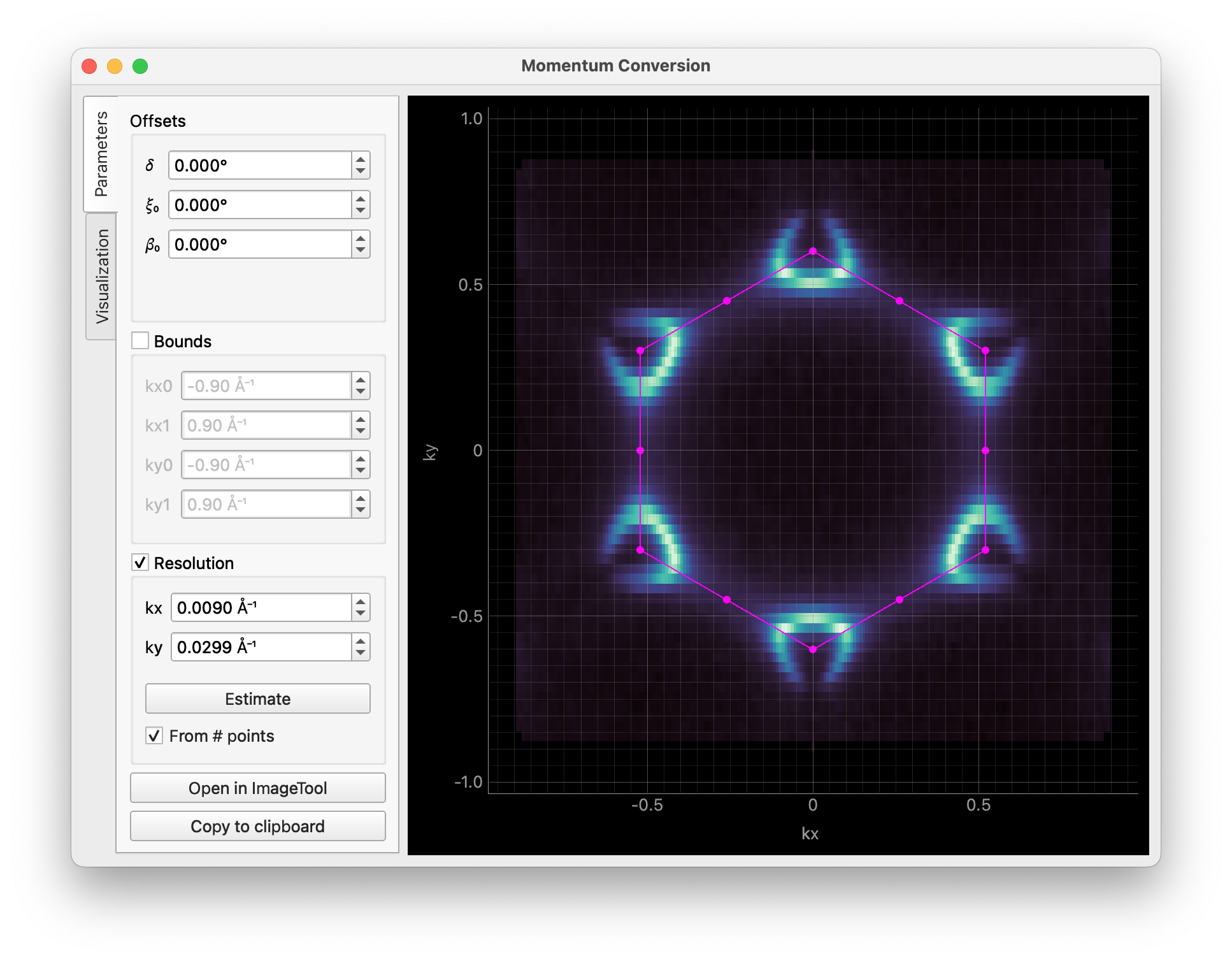
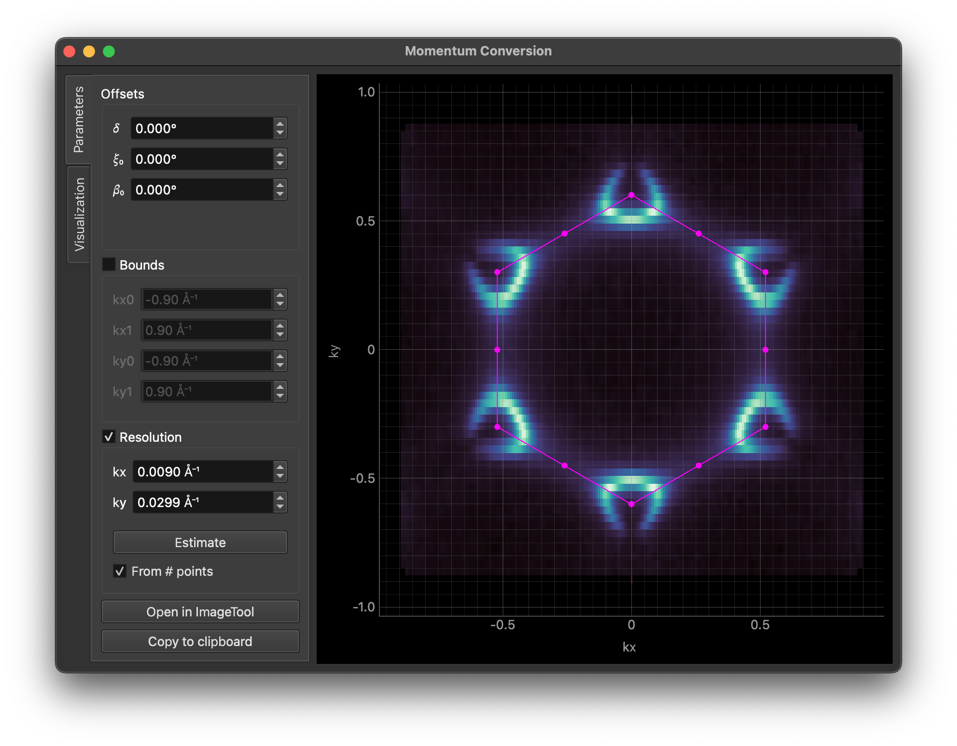
The first tab is for setting momentum conversion parameters. The image is updated in real time as you change the parameters. Clicking the “Copy code” button will copy the code for conversion to the clipboard. The “Open in ImageTool” button performs a full three-dimensional conversion and opens the result in the ImageTool.
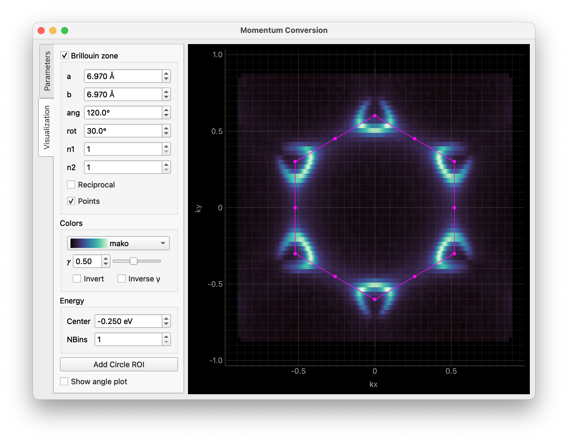
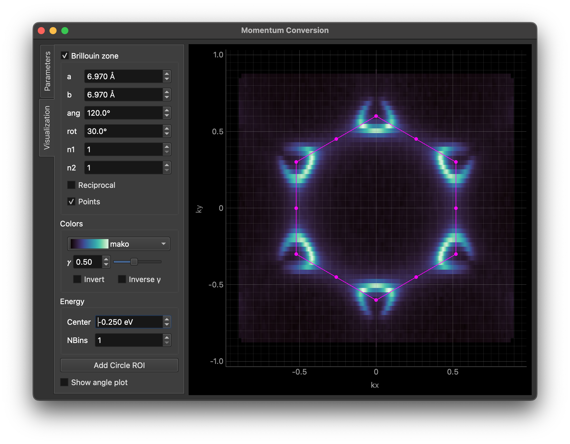
The second tab provides visualization options. You can overlay Brillouin zones and high symmetry points on the result, adjust colors, apply binning, and more. The “Add Circle ROI” button allows you to add a circular region of interest to the image, which can be edited by dragging or right-clicking on it.
You can pass some parameters to customize the GUI. For example, you can set the Brillouin zone size/orientation and the colormap like this:
data.kspace.interactive(
    avec=np.array([[-3.485, 6.03], [6.97, 0.0]]), rotate_bz=30.0, cmap="viridis"
)
See the documentation of erlab.interactive.ktool() for more information.