Filtering

Image processing-related functions are commonly used in the analysis of ARPES data. The erlab.analysis.image submodule provides a collection of functions that are useful for processing and analyzing images.

The module includes xarray wrappers for several functions in scipy.ndimage and scipy.signal, along with several processing methods that are commonly used to visualize ARPES data.s

Image smoothing filters

import erlab.analysis as era

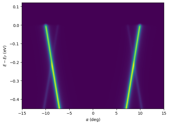
First, let us generate some example data: a simple tight binding simulation of graphene.

from erlab.io.exampledata import generate_data_angles

cut = generate_data_angles(
    shape=(500, 1, 500),
    angrange={"alpha": (-15, 15), "beta": (-5, 5)},
    seed=1,
    bandshift=-0.2,
).T
cut.qplot()

<matplotlib.image.AxesImage at 0x76f5da5be390>

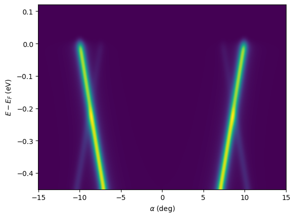
Here, we apply a Gaussian filter in coordinate units using erlab.analysis.image.gaussian_filter() to simulate an instrumental broadening of 10 meV and 0.2 degrees:

cut_smooth = era.image.gaussian_filter(cut, sigma=dict(eV=0.01, alpha=0.2))
cut_smooth.qplot()

<matplotlib.image.AxesImage at 0x76f5d3ea2720>

For all arguments and available filters, see the API reference at erlab.analysis.image.

Visualizing dispersive features

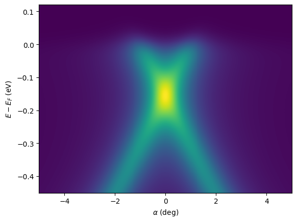
There are several methods that are used to visualize dispersive features in ARPES data. To demonstrate, we first generate a synthetic ARPES cut with broad features:

import erlab.analysis as era

from erlab.io.exampledata import generate_data_angles

cut = generate_data_angles(
    shape=(500, 1, 500),
    angrange={"alpha": (-5, 5), "beta": (-10, 10)},
    temp=200.0,
    seed=1,
    bandshift=-0.15,
    Simag=0.1,
    count=1e11,
).T
cut.qplot()

<matplotlib.image.AxesImage at 0x76f5d3c1ad20>

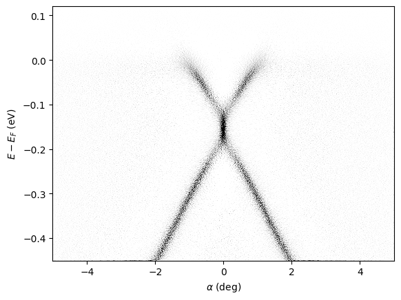
The 2D curvature can be calculated with erlab.analysis.image.curvature():

result = era.image.curvature(cut, a0=0.1, factor=1.0)

result.qplot(vmax=0, vmin=-200, cmap="Greys_r")

<matplotlib.image.AxesImage at 0x76f5d2d5e120>

For different methods and arguments, see the API reference at erlab.analysis.image.

Interactive differentiation

A GUI for interactive smoothing and differentiation can be invoked with erlab.interactive.dtool():

import erlab.interactive as eri

eri.dtool(cut)

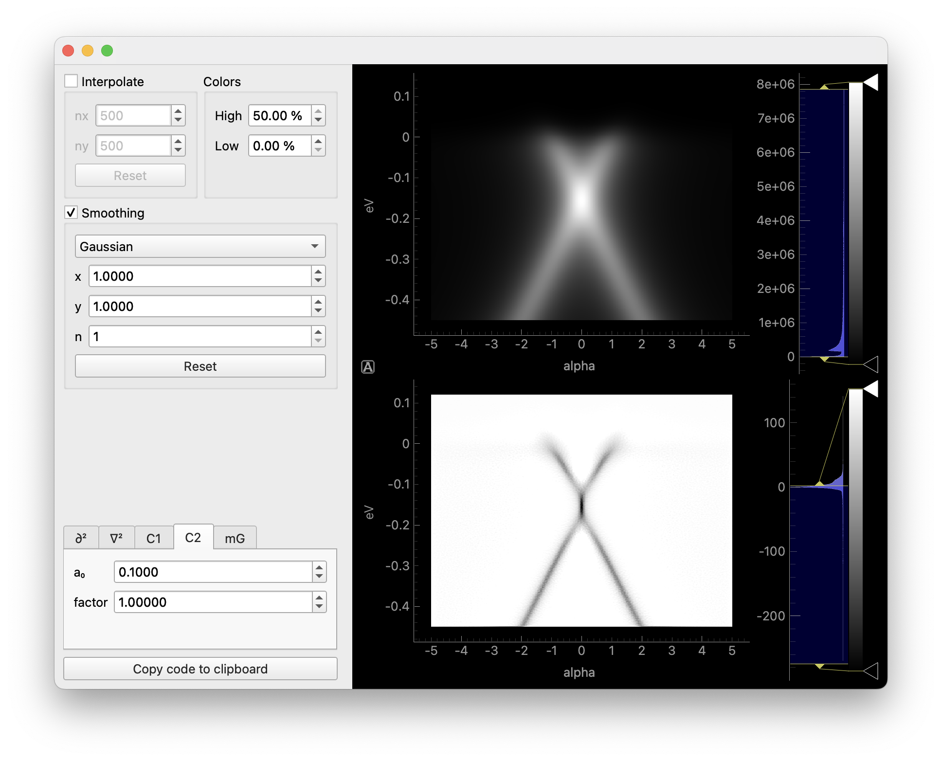
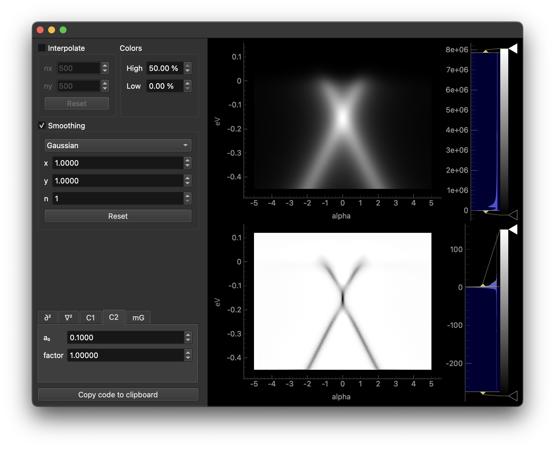
• The first section interpolates the data to a grid prior to smoothing.

• The second section applies Gaussian filtering prior to differentiation.

• In the third section, selecting different tabs will apply different methods. Each tab contains parameters relevant to the corresponding method.

• Clicking the copy button will copy the code for differentiation to the clipboard.

• Both the data and the result can be opened in ImageTool from the right-click menu of each plot, where it can be exported to a file.